Looking at a stack of flat, 2D medical scans is a lot like trying to understand a complex story by reading one page at a time. The real magic happens when you bind those pages together. That's precisely what 3D reconstruction from 2D images does—it stitches individual slices into a complete, interactive 3D model, adding the crucial dimension of depth that can transform a diagnosis.
Understanding the Core Challenge of 3D Reconstruction
At its heart, the goal is to recover spatial information that was lost when the image was captured. A 2D image is just a flat projection of a three-dimensional world. The entire point of 3D reconstruction is to use algorithms to rebuild that missing third dimension. For a clinician, this means taking a series of CT or MRI slices and computationally stacking them into a 3D volume they can actually manipulate.
This isn't just for show. It represents a fundamental shift in how doctors interact with patient data. They no longer have to mentally assemble anatomy from one slice to the next; they can see the entire structure at once, rotate it, and inspect it from any angle.
From Simple Illusions to AI-Powered Insights
Getting to this point has been a long road filled with major technical hurdles. Early attempts back in the mid-20th century were pretty basic, relying on stereoscopic tricks like the old-school anaglyphic 3D glasses from the 1950s to create a simple illusion of depth. The real game-changer was the explosion of machine learning in the 2010s.
Breakthroughs like Deep3D, developed in 2016, demonstrated how deep convolutional neural networks (CNNs) could automatically turn 2D images into stereoscopic 3D. This was a massive leap from clever optical illusions to true computational insight. If you're curious, it's worth taking a deeper look into the history of these conversion techniques to see just how far we've come.
Key Takeaway: Modern 3D reconstruction isn't about creating a pretty picture. It's about building a data-rich, interactive model that provides real clinical value for diagnostics, surgical planning, and patient education.
Why This Matters for Clinical Practice
The ability to perform accurate 3D reconstruction from 2D images delivers direct, tangible benefits in any healthcare setting. It turns passive data viewing into an active, exploratory process.
Here’s a snapshot of what that looks like in the real world:
- Improved Diagnostic Accuracy: Visualizing a tumor's exact size, shape, and relationship to surrounding blood vessels is infinitely easier in 3D.
- Enhanced Surgical Planning: Surgeons can rehearse a complex procedure on a patient-specific 3D model, which can help reduce operating times and improve outcomes.
- Better Patient Communication: Showing a patient a 3D model of their own anatomy is a powerful way to explain a condition or procedure, which helps with informed consent.
- Foundation for 3D Printing: These reconstructed models are the direct source files for 3D printing, allowing for the creation of physical anatomical models for planning or training.
This table breaks down the process into its essential stages, from raw data to a usable 3D model.
| Core Stages of the 3D Reconstruction Pipeline |
| :— | :— | :— |
| Stage | Objective | Key Challenge |
| 1. Data Acquisition & Preprocessing | Ingest and standardize 2D image slices (e.g., from DICOM files). | Handling inconsistent slice thickness, noise, and artifacts. |
| 2. Feature Extraction & Matching | Identify corresponding points or features across adjacent slices. | Ensuring accurate alignment, especially with patient movement. |
| 3. Volumetric Reconstruction | Use algorithms to stack and interpolate the aligned slices into a 3D grid. | Balancing computational cost with model resolution and accuracy. |
| 4. Surface Rendering & Visualization | Generate a viewable mesh or surface from the volumetric data. | Creating a medically accurate and visually intuitive representation. |
Each stage presents its own set of problems to solve, but the result is a powerful tool that was unimaginable just a few decades ago.
Throughout this guide, I'll give you a practical, hands-on roadmap for building your own AI-driven pipeline to do exactly this. We’ll cover everything from wrangling raw medical data to deploying a functional model, equipping you with the skills to turn flat scans into powerful clinical insights.
Mastering Your Data with a DICOM Workflow
Any successful 3D reconstruction from 2D images lives and dies by the quality of its data. In the medical field, that means getting really good at handling the DICOM (Digital Imaging and Communications in Medicine) standard. It's not enough to just have a folder full of .dcm files; you need a rock-solid workflow to transform that raw data into something your model can actually use.
This isn't just a "nice-to-have." It's a non-negotiable step that protects patient privacy, pulls out the critical details needed for an accurate reconstruction, and sidesteps the subtle errors that can poison your entire project. Think of it as laying the foundation for a house—if you get that wrong, everything you build on top will be unstable.
Navigating Anonymization and Metadata
First things first: before you do anything else, you absolutely must anonymize the data. Patient privacy is everything, and regulations like HIPAA are crystal clear about removing all Protected Health Information (PHI) from DICOM files. We're talking names, patient IDs, dates—all of it. Skipping this step isn't just sloppy; it's a major compliance risk.
Once your data is safely anonymized, it's time to dig into the DICOM headers. These headers are a goldmine of metadata, and this information is the key to accurately reconstructing the 3D model. They contain the geometric instructions your pipeline will follow.
You’ll want to zero in on a few key tags:
- Slice Thickness: This tells you the distance between each 2D slice. Without it, you have no idea how to space the images along the Z-axis, and your 3D volume will be distorted.
- Pixel Spacing: This gives you the real-world size of a single pixel. It’s how you convert abstract pixel coordinates into meaningful measurements, like millimeters.
- Image Position (Patient): This tag provides the exact XYZ coordinates of the top-left corner of each slice. It's essential for stacking the images in the correct spatial order.
- Image Orientation (Patient): This defines the direction of the image rows and columns, which helps you correctly interpret axial, sagittal, and coronal views.
A classic rookie mistake is just assuming all the slices in a folder are perfectly ordered and evenly spaced. I've seen it happen—scanner protocols glitch, or export processes jumble the files. Always, always use the DICOM metadata to verify the sequence and spacing.
From Raw Slices to Volumetric Data
With your metadata extracted, you can get to the main event: stacking the 2D slices into a single 3D volume. The process involves reading each DICOM file, grabbing its pixel data, and carefully placing it into a large 3D array (a NumPy array is perfect for this) based on the spatial information you just pulled from the headers.
This is where you lean on the power of open-source libraries. For instance, pydicom is a fantastic Python library built specifically for this. It lets you read, tweak, and write DICOM files without reinventing the wheel.
Tools like pydicom automate the grunt work of parsing headers and accessing pixel arrays, which saves a ton of time and prevents the kinds of manual errors that are all too easy to make.
Another workhorse is SimpleITK. It's designed for medical image analysis and has powerful functions for reading an entire DICOM series directly into a 3D volume. It even intelligently sorts the slices based on their spatial position, which is a common failure point when you try to do it by hand.
The ultimate goal here is to convert that messy folder of individual DICOM files into a single, clean file that your machine learning framework can easily handle. Formats like a NumPy array (.npy) or a NIfTI file (.nii.gz) are standard. The NIfTI format is especially popular in medical AI because it neatly packages both the 3D volume data and its spatial metadata (like voxel dimensions) into one place.
Of course, to build models that perform well, you need more than just clean data; you need well-labeled data. For many projects, this means getting high-quality image annotation to create the ground truth your model will learn from. This is especially true for supervised learning, where the model needs clear examples to understand what it's supposed to be finding.
By setting up a rigorous DICOM workflow from the start, you build a repeatable, reliable process for data prep. This disciplined approach is the first, and arguably most important, step toward building a successful AI model for 3D reconstruction from 2D images.
Choosing and Training Your Reconstruction AI
Alright, you've wrangled your DICOM data into shape. Now comes the exciting part—the engine of our entire pipeline. This is where we teach a machine to see a stack of flat, 2D images and intelligently build a 3D volume from them.
Picking the right AI model isn't about finding the "best" one. There's no such thing. The right choice depends entirely on what you're trying to accomplish. Are you isolating a specific organ, like a liver, to measure its volume? Or are you trying to generate a complete, photorealistic 3D model of the entire scanned area? These are two very different goals that lead to very different AI architectures.
The Two Main Paths: Segmentation vs. Direct Synthesis
Your first big decision is how the AI will approach the problem. In my experience, virtually all medical 3D reconstruction from 2D images falls into one of two camps: segmentation-based reconstruction or direct synthesis. Each has its place, and knowing the difference is key.
Segmentation-based reconstruction is often the most practical and reliable route for clinical work. It’s a two-step dance:
- First, you train an AI model—almost always a U-Net or a similar architecture—to go through each 2D slice and create a segmentation mask. Think of this as the AI "coloring in" the pixels that belong to the specific structure you're interested in, like a tumor or a particular bone.
- Next, you simply stack these 2D masks, one on top of the other, to create a 3D volume of just that object.
This method is so popular because it’s robust and gives you a clean, isolated model of a specific anatomical structure. It's easier to train, and the results are directly interpretable.
The other path is direct synthesis. Here, you’re asking the model to dream up the entire 3D volume at once from the 2D slices. This is a much heavier lift, typically tackled with complex models like Generative Adversarial Networks (GANs). A GAN works by pitting two networks against each other: a "generator" that creates 3D volumes and a "discriminator" that tries to tell the fake, generated volumes from real ones. Through this competition, the generator becomes incredibly skilled at producing high-fidelity results. The breakthroughs here are what have made single-image 3D reconstruction a reality. If you're curious about the deep tech, you can explore how GANs and NeRFs are pushing the boundaries on pycad.co.
Here’s a quick breakdown of how these two approaches stack up.
| Model Comparison | U-Net (Segmentation) | GAN (Direct Synthesis) |
|---|---|---|
| Primary Goal | Isolate specific anatomical structures. | Generate a complete 3D volume directly. |
| Data Requirement | Requires pixel-level annotated masks. | Needs paired 2D slices and 3D volumes. |
| Interpretability | High; the model's output is easy to understand. | Lower; can feel like a "black box." |
| Computational Cost | Generally lower during training. | Significantly higher, requires more GPU power. |
| Best For | Clinical tasks needing precise boundaries (e.g., tumor measurement). | Research or applications where realism is key. |
For most real-world clinical applications, a U-Net is going to give you the best bang for your buck in terms of performance and practicality.
Setting Up Your Training Pipeline
Once you've settled on an architecture, you have to define the rules for how it learns. This really boils down to three key components: a loss function, an optimizer, and a solid data augmentation strategy.
The loss function is what tells the model how far off its predictions are. This choice is critical. For a segmentation task, you might be tempted to use a standard loss like Cross-Entropy, but it often stumbles when dealing with the class imbalance common in medical images (think of a tiny tumor on a huge background of healthy tissue).
A much smarter choice for medical segmentation is the Dice Loss. It’s designed to measure the overlap between the predicted mask and the true mask, which makes it far more resilient to that kind of class imbalance.
Next, your optimizer is the algorithm that actually nudges the model's parameters in the right direction based on the loss. The Adam optimizer has become the default choice for a reason—it’s effective, stable, and works well out of the box. It’s the perfect place to start.
Pro Tip: While Adam is a fantastic default, don't be afraid to experiment a bit. I've found that optimizers like AdamW (which adds a concept called weight decay) can sometimes help the model generalize better and prevent it from just memorizing the training data.
Data Augmentation: Your Secret Weapon
Finally, let's talk about data augmentation. This is your most powerful tool, especially when you have a limited number of annotated medical scans. The idea is to apply random, realistic transformations to your training images, creating an almost infinite stream of new training examples. This forces your model to learn the true, underlying anatomy instead of just superficial image features.
For medical images, some of the most effective augmentations are:
- Elastic Deformations: This simulates the natural, non-rigid warping of soft tissue, making the model more robust to variations in patient anatomy.
- Gamma Correction: By tweaking image brightness and contrast, you teach the model to handle scans from different machines or with different settings.
- Random Rotations and Flips: These are simple but essential for making sure your model doesn't care if a patient was scanned in a slightly different orientation.
By carefully selecting your model, thoughtfully configuring your training loop in a framework like PyTorch or TensorFlow, and applying aggressive data augmentation, you'll forge a powerful and resilient AI. This model is the beating heart of your pipeline, ready to reliably perform the critical task of 3D reconstruction from 2D images.
Validating and Refining Your 3D Models

Getting a trained model to produce a visually impressive 3D rendering feels like a huge win, but let's be clear: it's not the finish line. For a 3D reconstruction from 2D images to have any real-world value, especially in a clinical setting, it needs to be rigorously validated. This isn't just about making sure it "looks good"—it's a systematic process to prove your model is both technically sound and clinically meaningful.
Think of validation as your essential quality control checkpoint. This is where you demonstrate that the 3D volume your AI generated isn't just some plausible-looking shape but a trustworthy representation of the patient's actual anatomy. Without this step, you’re flying blind and can't depend on the outputs for any serious application.
Establishing a Quantitative Baseline
The first layer of validation always starts with cold, hard numbers. You need objective metrics to measure how well your model's output stacks up against the "ground truth." In medical imaging, this ground truth is almost always a set of manual segmentations meticulously drawn by a clinical expert.
To do this right, you absolutely must use a dedicated, untouched hold-out test set. This is non-negotiable. This data must be completely new to the model, having never been used during training or any hyperparameter tuning.
Here are the standard metrics we rely on in the field:
- Intersection over Union (IoU): You might also hear this called the Jaccard index. It’s a straightforward measure of the overlap between your model’s prediction and the ground truth mask. A score of 1.0 is a perfect match, while 0.0 means no overlap whatsoever. It’s a fantastic all-around metric for segmentation accuracy.
- Dice Coefficient: Very similar to IoU, the Dice score is another overlap-based metric that's incredibly popular in medical imaging circles. Many find it a bit more intuitive for evaluating segmentations, particularly for smaller or more intricate structures.
- Hausdorff Distance: This one is different. It's less about overlap and more about boundaries. It calculates the greatest distance between any point on your predicted model's surface and the closest point on the ground truth surface. In essence, it tells you the worst-case error at the model's edge.
These scores give you an unbiased, objective way to compare different models or track your progress as you refine your approach. They are the foundation of any solid validation pipeline.
A Word of Caution: Never hang your hat on a single metric. A model could boast a high IoU but have a terrible Hausdorff Distance because it captured the general shape but missed a small, yet clinically vital, detail. Using a combination of metrics is the only way to get a complete picture of your model's performance.
The Indispensable Role of Qualitative Review
Numbers can't tell you the whole story. A model with a 95% Dice score might seem nearly perfect, but what if that 5% error consistently manifests as a hole in an artery wall? That's a catastrophic failure a simple score would never reveal. This is exactly why qualitative assessment—visual inspection by a subject matter expert—is absolutely critical.
This review process means sitting down with a clinician or radiologist and having them scrutinize the 3D reconstructions. They're not just looking at pretty pictures; they're hunting for specific problems that metrics can't see:
- Anatomical Plausibility: Does the heart actually look like a heart? Are there strange artifacts, unnatural holes, or floating, disconnected chunks of tissue?
- Boundary Smoothness: Are the surfaces smooth and continuous as they should be, or are they jagged and blocky?
- Clinical Relevance: Most importantly, does the model accurately capture the specific features a doctor needs to see? This could be the precise shape and volume of a tumor or the path of a complex vessel.
This human-in-the-loop feedback is priceless. It closes the gap between what is computationally "correct" and what is clinically useful, helping you pinpoint subtle but significant flaws in your model.
Post-Processing for a Polished Final Product
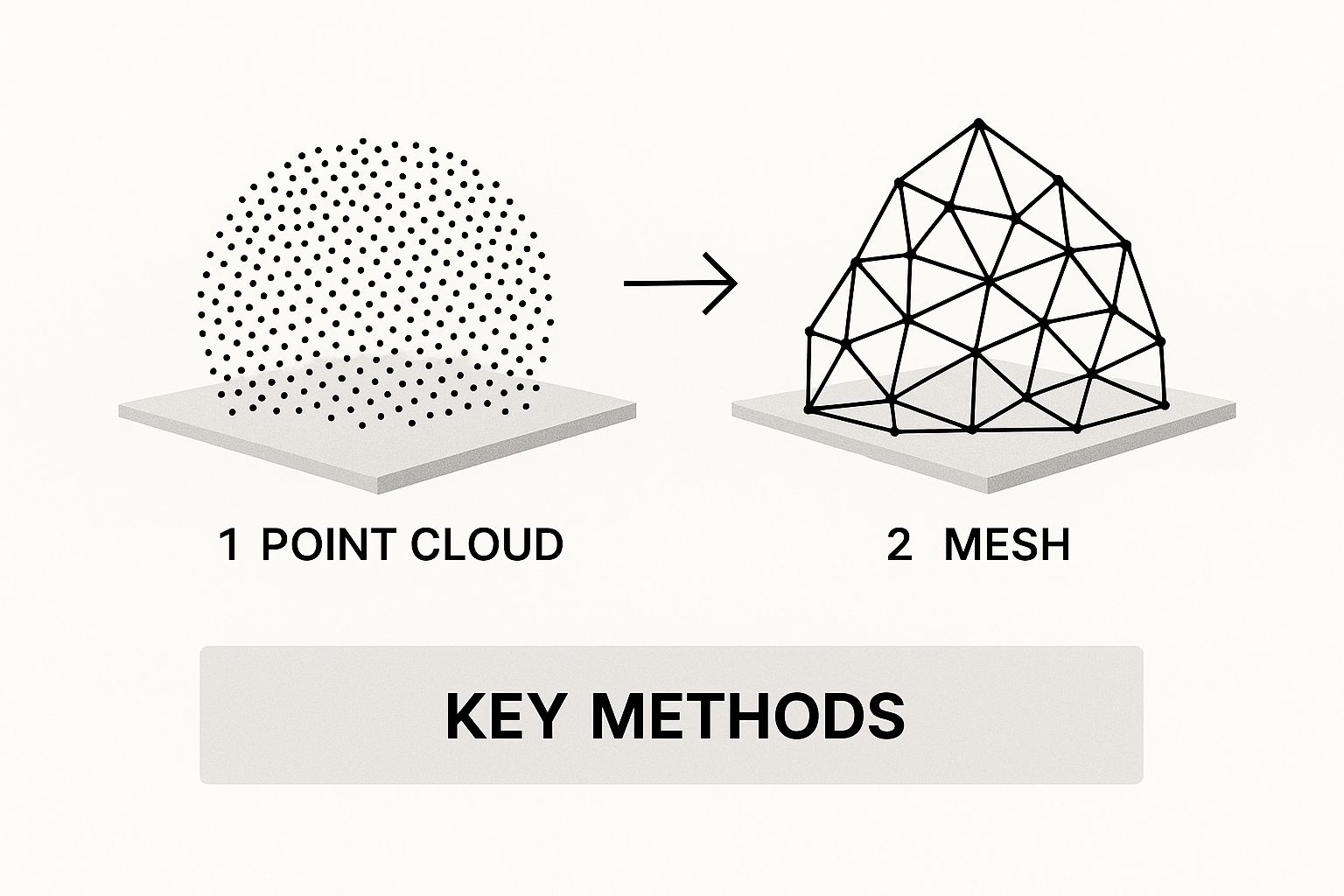
Once your model's core output has passed validation, it's time for the final refinement. The raw output from an AI model is usually a voxel grid—a 3D array of data points. To transform this into a smooth, render-ready 3D mesh you can use for visualization or 3D printing, you need to apply some post-processing.
The Marching Cubes algorithm is the industry-standard technique here. It works by "marching" through the voxel grid and converting the volumetric data into a triangulated surface mesh, which you'd typically save as an STL or OBJ file. This method is fundamental to many types of 3D modeling. In fact, many classic methods of 3D reconstruction from multiple 2D images rely on similar principles, like triangulation, to build a point cloud before meshing. You can explore more about this foundational technique on Wikipedia.
On top of that, applying smoothing filters like Laplacian or Taubin smoothing can work wonders. These help reduce the blocky, "stair-step" artifacts that are common in models derived from voxels. The filters gently average the positions of the vertices to create a more organic, visually appealing surface without messing with the underlying shape. This final polish is what makes your model not just accurate, but genuinely ready for real-world use.
Putting Your Model to Work in a Clinical Setting
Alright, you've trained and validated a fantastic model. It performs beautifully on your test data, and the metrics look great. Now comes the hard part: getting it out of the lab and into the hands of a clinician. This is where many projects hit a wall, because a model that's brilliant in theory is useless until it's a practical, usable tool.
Moving to deployment means shifting your focus from pure accuracy to real-world considerations like speed, usability, and how your tool fits into an already complex hospital workflow. This final step is what turns all your research and development on 3D reconstruction from 2D images into something that can genuinely help people.
Designing an Interface for Clinicians, Not Coders
First things first, clinicians need an interface. They're experts in medicine, not command-line prompts. Your goal is to give them a simple, intuitive tool that feels like a natural part of their day, not an extra chore.
A great starting point for internal testing and getting quick feedback is a web-based UI. I'm a big fan of using a framework like Streamlit for this. You can spin up a functional app surprisingly fast, letting a radiologist upload a DICOM series and see the resulting 3D model in minutes. It's the perfect way to prototype without sinking months into development.
But for a truly seamless, long-term solution, you'll want to build a plugin for the software they already use every day. Think about integrating directly into widely used medical image viewers like 3D Slicer or ITK-SNAP. When your model becomes a feature inside a program they already trust, you've effectively removed the biggest barrier to adoption.
I’ve seen projects stall because the final tool was too clunky or required too many extra steps. The goal should always be to make your model feel like a native feature of the clinician's existing software, not a separate, cumbersome application they have to switch to.
Choosing Your Deployment Strategy
Next, you have to decide where your model will actually run. This decision has huge implications for cost, speed, and, most importantly, patient data security. You're generally looking at two paths, each with its own pros and cons.
- Local Deployment: Here, the model runs directly on the clinician's own workstation. This is fantastic for data privacy, as sensitive patient information never leaves the local machine. The downside? Every single workstation needs a powerful enough GPU to handle the load, and rolling out updates across an entire department can be a logistical headache.
- Server-Based Deployment: In this setup, the model lives on a central server, either on-premise or in the cloud. The clinician’s computer sends the anonymized 2D images to the server, which does the heavy lifting and sends the finished 3D model back. This centralizes your hardware needs and makes updates a breeze, but you have to account for network latency and navigate more complex data security and governance rules.
For healthcare organizations, this choice often comes down to their existing IT infrastructure and whether they have the right team in place. The challenges of hiring AI talent for healthcare are very real, and having the right people on board can heavily influence which deployment strategy makes the most sense.
Optimizing for the Real World: Speed and Compatibility
Let's be realistic: a model that takes 30 minutes to reconstruct a volume won't fly in a busy clinic. Inference speed is everything. This is where you need to optimize your model for performance. A standard best practice is to convert your model from its training format (like PyTorch’s .pt file) to a universal, high-performance format like ONNX (Open Neural Network Exchange).
The ONNX Runtime is built specifically for fast inference across different types of hardware. Just this one conversion step can often give you a massive performance boost—I've seen it make models 2-3x faster without changing a single line of the model's architecture.
Finally, think about the finish line: the output file. Your pipeline needs to generate a 3D model in a format that other clinical applications can actually open and use.
Common Output Formats and Their Uses:
| Format | File Extension | Primary Use Case |
|---|---|---|
| STL | .stl |
The gold standard for 3D printing anatomical models. |
| OBJ | .obj |
Great for surgical planning software and advanced visualization. |
| PLY | .ply |
Useful for storing 3D scanner data, especially with color. |
Making sure your model outputs a clean, compatible file—an STL for the 3D printer or an OBJ for the surgical planning suite—is the final piece of the puzzle. It’s this attention to practical detail that transforms a powerful AI algorithm into a truly valuable clinical asset.
Answering Your Top Questions on Medical 3D Reconstruction
When you start diving into 3D reconstruction from 2D medical images, a few questions almost always come up. Getting these sorted out from the get-go can save you a world of headaches down the road. Let's walk through some of the most common queries I hear from teams tackling these projects.
How Much Data Do I Really Need?
This is the classic "it depends" question, but I can give you some solid guideposts. The amount of data you'll need is completely tied to the complexity of your model and how much detail you're trying to achieve.
If you’re taking a segmentation-first approach with something like a U-Net, you can often get a decent start with several dozen high-quality, expertly annotated scans. The real bottleneck here isn't the number of scans but the quality of the annotations—that's what the model is learning from.
On the other hand, if your goal is direct synthesis using a more sophisticated generative model like a GAN, you're looking at a much bigger data requirement. You'll likely need hundreds of scans to train a model that can generate convincing and accurate volumes. No matter which path you choose, aggressive data augmentation is non-negotiable, especially when your dataset is on the smaller side.
Can I Just Use a Standard Pre-Trained Model?
It’s always tempting to grab a model that’s been pre-trained on a huge dataset like ImageNet and see what happens. This is called transfer learning, and while it's a great starting point for basic feature extraction, it's almost never the final answer for medical imaging.
Why? Medical scans are just built differently from regular photos. Their statistical properties—the grayscale values, the specific textures of human tissue, the unique imaging artifacts—are a world away from pictures of cats and dogs.
My Experience: A model that's an expert at identifying cars simply doesn't have the built-in knowledge to understand the subtle gray-on-gray differences in a CT scan. You will absolutely need to do some serious fine-tuning on a relevant medical dataset to get anywhere near the accuracy needed for real-world use.
What’s the Biggest Hurdle in Clinical Deployment?
Getting a model to work in the lab is one thing; getting it into a live hospital workflow is a completely different ballgame. While technical issues like inference speed and integrating with PACS systems are real challenges, they’re usually not the main event.
From my experience, the biggest obstacles are almost always:
- Regulatory Approval: Securing clearance from bodies like the FDA in the US or a CE mark in Europe is a marathon, not a sprint. It’s an incredibly rigorous process demanding exhaustive documentation and validation.
- Building Clinician Trust: At the end of the day, doctors have to trust your model. You build that trust through transparent performance metrics, being upfront about the model’s limitations, and showing how it genuinely improves upon their current tools.
What’s the Difference Between Surface and Volume Rendering?
These are two common ways to visualize the 3D data your model creates, and each has its own place. Think of them as different tools for different jobs.
Surface rendering first creates a geometric mesh of an object's surface, often using an algorithm like Marching Cubes, and then renders that mesh. It's computationally efficient and great for creating those clean, solid-looking models you might use for 3D printing or just to see the shape of an organ.
Volume rendering, in contrast, works directly with the raw data. It assigns a color and an opacity level to every single voxel in your 3D grid. This technique lets you create those beautiful, semi-transparent visualizations where you can see internal structures and how different tissues overlap. It’s perfect for getting a feel for the spatial relationships within the anatomy.
Ready to build your own advanced medical imaging solutions? PYCAD specializes in the entire AI pipeline, from data handling and model training to final deployment. We help you turn complex 2D scans into actionable 3D insights. Find out how we can accelerate your project.