Data Preprocessing for Machine Learning: Essential Techniques

Think of data preprocessing as the essential prep work before you start cooking a gourmet meal. It’s the process of cleaning, transforming, and organizing raw data until it’s in a perfect, high-quality format that a machine learning algorithm can actually understand and learn from.

This step is non-negotiable. Why? Because even the most powerful AI will produce garbage results if it's fed inconsistent, incomplete, or just plain "noisy" data.

The Hidden Engine of Successful Machine Learning Models

Imagine trying to build a high-performance engine with rusty, mismatched parts. No matter how brilliant the engineering design is, that engine would sputter and fail. Machine learning models work exactly the same way. Raw data, pulled from real-world sources, is almost always messy and completely unsuitable for direct use.

This is where data preprocessing becomes the critical engine room where models are either made or broken. It’s not just some preliminary task you check off a list; it's the foundational work that dictates whether everything else will run smoothly. Just as a master chef meticulously washes, chops, and measures ingredients before ever turning on the stove, a data scientist must get their hands dirty cleaning, transforming, and structuring raw data before feeding it to an algorithm.

Why Preprocessing Is Non-Negotiable

Without this careful preparation, a model's performance will nosedive. Algorithms are incredibly powerful but also stubbornly literal—they don't have the human intuition to ignore a typo or figure out that "N/A" and "0" might mean two totally different things. They need clean, consistent, and numerical input to do their job properly.

The quality of your input data directly dictates the quality of your output. Garbage in, garbage out isn't just a catchy phrase; it's a fundamental law in machine learning.

This foundational work is what directly boosts a model's accuracy, reliability, and overall performance. Seeing how successful companies use clean, well-structured data to drive their systems really hammers home its importance. For instance, understanding how Amazon personalizes product recommendations reveals the immense power of high-quality data in building effective, real-world AI.

This guide will walk you through the essential stages of preprocessing, setting you up with the practical techniques needed to turn chaotic raw information into a truly valuable asset.

Key Stages in the Preprocessing Pipeline

The whole process can be broken down into a few core stages, with each one tackling a different kind of data imperfection. Think of these as the backbone of any serious machine learning project.

• Data Cleaning: This is all about handling missing values, correcting inconsistencies, and smoothing out noisy data. It's the digital equivalent of tidying up.
• Data Transformation: Here, we're scaling features to a common range, encoding categorical variables (like "Red" or "Blue") into numerical formats, and normalizing data distributions.
• Feature Engineering: This is where the creativity comes in. It's the art of creating new, more informative features from the existing data to give your model more to work with and boost its performance.
• Data Splitting: The final step. We carefully divide our pristine dataset into training, validation, and test sets. This is how we properly evaluate our model's ability to generalize to new, unseen data.

Why Raw Data Will Sabotage Your Models

Feeding raw, unprocessed data directly into a machine learning algorithm is a recipe for disaster. Think of it like trying to build a house on a foundation of quicksand. No matter how sophisticated your architecture or how skilled your builders, the entire structure is destined to fail.

Machine learning models are powerful, but they are also incredibly literal. They have zero intuition. They can't guess what you meant or infer context from messy inputs. This is why raw data will actively sabotage your models—it’s filled with traps that can mislead, confuse, or completely break an algorithm.

This is where the real work begins. The meticulous process of cleaning and preparing your data is the cornerstone of effective data preprocessing for machine learning, and it’s what separates successful projects from failed experiments.

The Anatomy of a Messy Dataset

Real-world data is never as clean as the textbook examples. It's often riddled with problems that can silently corrupt your results. Getting a handle on these common culprits is the first step toward building a model you can actually trust.

Here are the four usual suspects you'll need to deal with:

• Missing Values: Gaps in your data, often showing up as NaN or null, can make many algorithms crash. If they don't crash, they might produce skewed, unreliable results.
• Inconsistent Formats: Imagine a single column with dates written as "10-25-2023", "25/10/23", and "Oct 25, 2023". A human can figure it out, but a model sees chaos.
• Outliers: These are the extreme data points that don't fit the pattern. A single typo can create an outlier that pulls your entire model in the wrong direction.
• Imbalanced Scales: If one feature is "age in years" (e.g., 25, 40, 65) and another is "income in dollars" (e.g., 50000, 90000, 120000), the model will naturally give more weight to the income figures simply because the numbers are bigger.

Let’s say you’re building a sales forecasting model. A single data entry error records a sale of $1,000,000 instead of $1,000. To the algorithm, that’s not a mistake; it's a massive, legitimate sale. This one outlier could cause the model to wildly overestimate all future revenue, rendering it useless.

The True Cost of Neglecting Preprocessing

Skipping this step leads to everything from slightly inaccurate predictions to completely nonsensical outcomes. A model trained on messy data might look great on paper, but it will almost certainly fall apart when it encounters new information from the real world. It has learned all the noise, errors, and quirks instead of the actual patterns you wanted it to find.

The reality of data science is that meticulous preparation is not just a preliminary step—it's the main event. Turning potential data disasters into reliable insights is where the bulk of the work happens.

This isn't just a gut feeling. Industry reports consistently show that data scientists spend a massive chunk of their time—often 60-80%—just cleaning and organizing data. You can find a deeper dive into these industry findings on data preparation on TechTarget. That huge time investment is what it takes to remove the noise, fix the inconsistencies, and ultimately build a model that works.

Building a Strong Foundation

Every technique we'll cover, from handling missing values to scaling features, is designed to solve a specific problem lurking in raw data. By systematically addressing these issues, you transform a chaotic mess into a structured, high-quality asset your model can actually learn from.

This transformation is non-negotiable. It allows the algorithm to focus on what truly matters: the meaningful relationships and patterns hidden within your data. Without this clean foundation, any insights you generate are built on shaky ground, ready to collapse at the first sign of real-world complexity.

Essential Techniques for Cleaning and Transforming Data

Now that we understand why raw data can be so troublesome, it’s time to roll up our sleeves and get to work. This is where the practical, hands-on side of data preprocessing for machine learning truly begins. We’re going to walk through the core techniques for fixing imperfections and reshaping your dataset into a clean, reliable format that machine learning algorithms can actually understand.

Think of yourself as a craftsman in a workshop. Your raw data is the block of wood—it has potential, but it's rough, uneven, and full of knots. Your job is to use the right tools to sand, cut, and shape it until it’s perfectly prepared for the final assembly. Each technique we'll cover is a different tool for a specific problem, from filling in gaps to leveling out skewed measurements.

Taming Missing Data with Imputation

One of the first and most common headaches you'll run into is missing data—those frustrating empty cells in your spreadsheet, often shown as NaN (Not a Number). You can't just ignore them; they can crash your code or, even worse, quietly introduce bias into your model. The process of intelligently filling in these gaps is called imputation.

There are a few solid ways to handle this, each with its own pros and cons:

• Mean/Median Imputation: This is the most straightforward approach. For any numeric column with gaps, you simply fill them with either the mean (average) or the median (the middle value). A good rule of thumb? Use the median if you suspect outliers are present, as it’s far less sensitive to extreme values.
• Mode Imputation: When you're dealing with categorical (non-numeric) data, like "Color" or "City," this is your go-to. You just find the mode—the value that appears most often—and use it to fill in the blanks.
• Constant Value Imputation: Sometimes, the fact that data is missing is itself a signal. In these cases, you can fill the gaps with a specific constant, like 0 or -1. This allows the model to potentially learn that the absence of a value is meaningful.

The right choice really depends on your dataset and what you’re trying to achieve. Simple imputation is often a great first step to get things moving.

Managing Outliers to Prevent Skewed Results

Outliers are those data points that just don't fit in. They're the anomalies, the values that are wildly different from everything else. They could be legitimate extreme cases or simple data entry mistakes, but either way, they can seriously warp your model's understanding of the data. Finding and dealing with them is non-negotiable for building a reliable model.

This is where basic statistics become your best friend, giving you metrics like mean and standard deviation to spot abnormalities. Outliers can drag your model’s predictions way off course by distorting the patterns it’s trying to learn. You can dive deeper into how statistical methods support data preprocessing on Neptune.ai.

A classic and highly effective method for finding outliers is using the Interquartile Range (IQR). It sounds complex, but the idea is simple:

1. Find the first quartile (Q1), the point where 25% of the data lies below it.
2. Find the third quartile (Q3), the point where 75% of the data lies below it.
3. Calculate the IQR, which is just Q3 – Q1.
4. Establish an "acceptable" range for your data, which is typically from Q1 - 1.5 * IQR on the low end to Q3 + 1.5 * IQR on the high end.
5. Any data point that falls outside this range is flagged as a potential outlier.

Once you’ve found them, you have a few choices: remove them, cap their values at the edge of your acceptable range, or apply a transformation to the data to lessen their impact.

Leveling the Playing Field with Feature Scaling

Imagine you’re building a model with two features: a person's age (from 18 to 90) and their annual income (from $30,000 to $250,000). Many algorithms, especially those that calculate distances like K-Nearest Neighbors (KNN), will naturally give more weight to income just because the numbers are so much bigger. The model becomes biased, thinking income is more important than age simply due to its scale.

Feature scaling fixes this by putting all your numerical features on the same scale, ensuring no single feature unfairly dominates the learning process.

It’s like trying to compare a distance measured in miles to one measured in millimeters. It’s impossible to do it fairly without first converting them to a common unit. Scaling does exactly that for your data.

Two primary techniques are used everywhere:

• Standardization (StandardScaler): This method re-centers your data to have a mean of 0 and a standard deviation of 1. It’s an excellent choice if your data roughly follows a bell curve (a Gaussian distribution) and is pretty robust against outliers.
• Normalization (MinMaxScaler): This technique squeezes your data into a fixed range, usually 0 to 1. It's especially handy for algorithms like neural networks that don't make assumptions about the data's distribution.

To make the choice clearer, here’s a quick comparison of these two popular scaling methods.

Comparing Feature Scaling Techniques

Technique	Method	Output Range	When to Use	Sensitivity to Outliers
Standardization	Subtracts the mean and divides by the standard deviation.	Centered around 0; no specific min/max.	When the data has a Gaussian (normal) distribution. Works well with algorithms like SVM and Logistic Regression.	Less sensitive than Normalization, but extreme outliers can still influence the mean and standard deviation.
Normalization	Scales values to a fixed range, typically 0 to 1.	Usually [0, 1] or [-1, 1].	For algorithms that do not assume a specific data distribution, like K-Nearest Neighbors (KNN) and neural networks.	Highly sensitive. A single outlier can drastically shrink the range of the rest of the data.

Choosing the right scaling technique isn't just a technical step—it's about understanding your data and the algorithm you plan to use. Standardization is often a safer default, but Normalization can be powerful when you know your data is bounded.

The infographic below highlights two other essential transformation techniques, this time for handling categorical data.

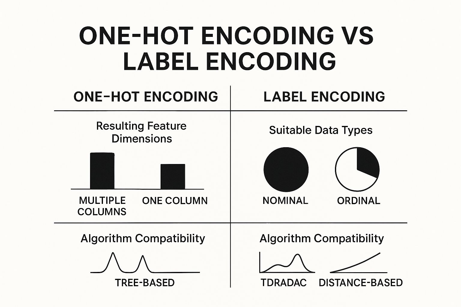
As you can see, One-Hot Encoding is perfect for nominal data (where categories have no order) because it creates new columns, while Label Encoding works best for ordinal data by assigning a single, ordered numerical value.

Getting Your Model to Understand Categories

Machine learning models are mathematical beasts. They thrive on numbers but get completely stumped by text. This becomes a real hurdle in data preprocessing for machine learning when you have datasets full of categorical features—think columns like 'Country', 'Product Category', or 'Patient Status'. You can't just throw text at an algorithm and hope for the best.

The answer is encoding, a process that translates these text labels into a numerical language your model can actually work with. Think of it like being a translator at the UN: you're converting one language (text) into another (numbers) so the conversation can move forward. The two most common tools for this job are One-Hot Encoding and Label Encoding.

Picking the right one is crucial. A wrong move here can accidentally introduce a false order or relationship into your data, leading your model down a completely wrong path.

One-Hot Encoding: When Order Doesn't Matter

Let's say you have a 'Color' feature with three options: 'Red', 'Green', and 'Blue'. If you just assigned them numbers—say, 1, 2, and 3—your model might get the wrong idea. It could mistakenly conclude that 'Blue' (3) is somehow "more" or "greater than" 'Red' (1), which is meaningless. This is the classic problem with nominal data, where the categories are just labels with no inherent ranking.

One-Hot Encoding neatly sidesteps this issue by creating a brand new binary (0 or 1) column for each category. For our 'Color' example, it would split that one column into three new ones: is_Red, is_Green, and is_Blue.

• An item that is 'Red' would get a 1 in the is_Red column and a 0 in the other two.
• An item that is 'Green' would get a 1 in the is_Green column and 0s elsewhere.

This way, the model sees each color as a distinct, independent entity without any implied hierarchy. It's the go-to method when your categories are just labels.

One-Hot Encoding is all about preventing your model from inventing a false order between categories. It treats every option as its own feature, which is vital for the integrity of nominal data.

But there's a catch. If your feature has a ton of unique categories (imagine a 'City' column with hundreds of cities), this method will explode your dataset with hundreds of new columns. This is known as the curse of dimensionality, and it can seriously slow down training and make your data much harder to manage.

Label Encoding: When Order Is Everything

Now, what if your categories do have a natural order? We call this ordinal data. A feature like 'T-Shirt Size' with values 'Small', 'Medium', and 'Large' has a clear progression. For cases like this, Label Encoding is the perfect fit.

Label Encoding works by assigning a simple integer to each category based on its rank. For our t-shirt sizes, the mapping would look something like this:

• 'Small' -> 0
• 'Medium' -> 1
• 'Large' -> 2

This is exactly what we want the model to see. The numerical relationship (0 < 1 < 2) mirrors the real-world relationship between the sizes, giving the model a powerful and accurate signal to learn from. It’s also very efficient, converting the feature into just one numerical column and avoiding the dimensionality problem entirely.

How to Make the Right Choice

Deciding between these two encoding methods comes down to answering one simple question: "Does the order of my categories mean something?"

1. If NO (Nominal Data): The categories are just distinct labels like 'Country' or 'Brand'. You should absolutely use One-Hot Encoding to avoid creating a fake hierarchy.
2. If YES (Ordinal Data): The categories have a meaningful rank, like 'Low', 'Medium', 'High' or 'Good', 'Better', 'Best'. Label Encoding is your tool, as it preserves that crucial sequential information.

Making the wrong call can really sabotage your model. If you used Label Encoding on a 'Country' column, you might teach your model that 'Canada' (say, encoded as 10) is somehow mathematically superior to 'Austria' (encoded as 3), which is just plain wrong. By translating your categorical data the right way, you ensure your model learns from real patterns, not from numerical noise you accidentally created.

From Raw Data to Rich Features: Engineering and Splitting

https://www.youtube.com/embed/SjOfbbfI2qY

Once you've cleaned up all the messy, missing, and inconsistent data, the real fun begins. This next part is where data preprocessing shifts from a science into an art form. You're no longer just tidying up; you're actively shaping the data to give your model the best possible chance to succeed.

This is the world of feature engineering, and it’s all about creatively crafting new, more powerful features from the ones you already have. Think of your raw data as a pile of ingredients. Sure, you have flour, sugar, and eggs, but that’s not a cake. Feature engineering is the chef's touch—combining those raw ingredients to create something far more valuable than the sum of its parts.

The Art of Creating New Features

The whole point of feature engineering is to pull out hidden signals from your data and serve them to your model on a silver platter. When you do this right, you can see a dramatic jump in your model's predictive power.

For instance, a simple timestamp column doesn't tell a model much on its own. But with a little creativity, you can engineer a goldmine of new features from it:

• Temporal Features: Isolate the hour of the day, the day of the week, or the month. This can instantly reveal powerful patterns, like e-commerce sales spiking on weekends or website traffic peaking after work hours.
• Interaction Features: Sometimes, two features are more powerful together. In a housing price model, simply multiplying the number of bedrooms by the total square footage might create a brand new feature that better captures a home’s usable living space.

This creative step is often what separates a decent model from a truly great one. In the financial sector, this isn't just a nice-to-have; it's essential. The global AI in banking market hit $19.9 billion in 2023 and is on track to explode to $315.5 billion by 2033. The banks that get this right—the ones adopting modern machine learning with sophisticated feature engineering—have reported sales increases of up to 10% on new products. You can dive deeper into the financial impact of machine learning on itransition.com.

The Most Important Step Before Training: Splitting Your Data

With your shiny new features in place, there's one final, non-negotiable step before you can start training: splitting your data. This is arguably one of the most critical moments in the entire machine learning workflow because it's the foundation for honestly evaluating your model's performance.

You need to break your dataset into distinct parts:

• Training Set: This is the lion's share of your data, typically 70-80%, that the model actually learns from.
• Validation Set: An optional slice of data used to fine-tune your model's parameters as you build it.
• Test Set: This is the protected 10-20% of your data. It stays locked away until the very end and is used only once to get an unbiased grade on how the model will perform on brand-new, unseen data.

Think of it like studying for a big exam. The training set is your textbook and notes. The validation set is the series of practice quizzes you take along the way. The test set is the final, proctored exam. You'd never peek at the final exam questions while studying—that's cheating.

Avoiding the Silent Killer: Data Leakage

That analogy brings us to a catastrophic but surprisingly common mistake: data leakage. This happens when information from outside the training set accidentally contaminates the model during its training phase. It’s the data science equivalent of giving your model the answers to the test.

The most common way this happens is when you perform preprocessing steps—like scaling features or filling in missing values—on the entire dataset before you split it. When you do that, information from the test set (like its overall average or maximum value) "leaks" into the training process. Your model will look like a genius during development, posting incredible accuracy scores, only to fail spectacularly in the real world.

To avoid this silent model killer, tattoo this golden rule onto your brain: Split first, preprocess second.

1. Split your raw data into training and test sets. Make this the very first thing you do.
2. Fit your scaler, imputer, or encoder only on the training data. Let it learn the patterns from that set alone.
3. Transform both the training and the test sets using that fitted preprocessor.

By truly mastering feature engineering and committing to a strict data splitting discipline, you build models that aren't just accurate on paper. You build models that are robust, reliable, and ready to deliver real value when it matters most.

Preprocessing Questions I Hear All the Time

As you start getting your hands dirty with data preprocessing, you'll quickly find it’s more of an art than a science. A lot of decisions feel subjective, and it's easy to get stuck wondering if you're making the right call. It’s totally normal.

Let's walk through some of the most common questions that pop up. Think of this as a field guide for those "what do I do now?" moments, based on years of seeing what works and what doesn't.

What’s the Single Most Important Preprocessing Step?

This is probably the number one question I get, but the honest answer is: it depends. There's no silver bullet. The "most important" step is whichever one fixes the biggest problem in your specific dataset for the model you’re using.

That said, two steps consistently have an outsized impact on performance.

First, handling missing data is almost always mission-critical. If you just ignore missing values, you’re either going to get errors or, worse, a biased model. Your model can only learn from the data you give it, and big gaps can completely warp its understanding of reality.

Second, for a huge number of algorithms, feature scaling is non-negotiable. Think about models that measure distance, like Support Vector Machines (SVMs), K-Nearest Neighbors (KNN), or even neural networks. They're incredibly sensitive to the scale of your features. Without scaling, a feature like salary (in the tens of thousands) will completely drown out a feature like years of experience (single or double digits). The model just won't work correctly.

While every step plays a role, getting missing data or scaling wrong can single-handedly tank an otherwise perfect model. The damage is direct, immediate, and often severe.

So, where do you start? Find the biggest, most obvious flaw in your raw data. That’s your most critical step.

How Do I Choose an Imputation Method?

Figuring out how to fill in missing data is a classic challenge. The best approach really boils down to what kind of data you have and how much of it is actually missing.

Here's a practical way to think about it:

• Just a few missing numbers? Go with mean or median imputation. It’s fast and usually gets the job done. A pro tip: use the median if you have outliers, since it isn't skewed by extreme values the way the mean is.
• Missing categories? The standard move here is to use the mode (the most frequent category). It's simple and effective.
• Lots of missing data? This is where it gets tricky. If a large chunk of data is gone, simple imputation can introduce some serious bias. You'll want to reach for something more sophisticated:
  • K-Nearest Neighbors (KNN) Imputation: This is a clever approach. It looks at the 'k' most similar rows (based on the other features) and uses their average value to fill the gap.
  • Model-Based Imputation: You can actually train a mini-model, like a linear regression, just to predict the missing values based on the other columns.

My advice? Start simple. Mean, median, or mode is often good enough and gives you a solid baseline to work from.

Can Preprocessing Actually Introduce Bias?

Oh, absolutely. This is something every data scientist needs to be hyper-aware of. Preprocessing isn't a neutral, mechanical task. Every choice you make can accidentally bake bias into your model, which can have very real consequences, especially in areas like healthcare or finance.

Imagine you're building a model for loan approvals. If you fill in missing income data using the overall average income from your dataset, you might be unintentionally erasing real-world income gaps between different demographic groups. Your model might end up being less fair or accurate for certain people.

Another classic example is outlier removal. In fraud detection, those "outliers" are often the exact transactions you're trying to find! If you toss them out because they look weird, you’re essentially training your model to ignore the very thing it's supposed to detect.

To fight this, always document every single preprocessing decision and think critically about the potential fallout. Ask yourself, "Could this choice distort how the data represents the real world?" Building a fair model is just as crucial as building an accurate one.

What Is Data Leakage and How Do I Stop It?

Data leakage is one of the sneakiest and most frustrating problems in machine learning. It happens when information from your test set—the data you've set aside to judge your final model—accidentally contaminates your training process.

The result? Your model looks like a genius during testing, with fantastic performance scores. But the moment you deploy it on truly new data, its performance completely collapses. It had a "cheat sheet" all along.

The most common way this happens is by doing your preprocessing on the entire dataset before splitting it. For example, if you calculate the mean to fill missing values using all your data, you’ve let your training process learn something about the test data's distribution.

The fix is surprisingly simple, but you have to be disciplined about it: Split first, preprocess second.

1. Split your data into training and test sets. Do this first. Always.
2. Fit your scalers, imputers, or encoders using only the training data. You're learning the "rules" from this set.
3. Transform both the training set and the test set using the rules you just learned.

This strict separation guarantees your test set remains 100% unseen, giving you a true, honest measure of how well your model will perform out in the wild.

---

At PYCAD, we live and breathe the complexities of medical imaging data, where a single preprocessing misstep can make the difference between a useless model and a life-saving one. From DICOM anonymization to deploying robust diagnostic AI, we manage the entire pipeline. Discover how PYCAD can advance your medical imaging projects.