Evaluating a machine learning model is how we figure out if it's actually any good. It’s the process of testing the model on data it has never seen before to check its accuracy, reliability, and ultimately, whether it works in the real world.
This isn't just a final exam. Think of it as a continuous reality check, making sure the model can generalize its knowledge—applying what it learned to new situations—rather than just "cramming" and memorizing the training examples. It's the only way to build models that people can trust and that actually solve the problem they were designed for.
Why Bother with AI Model Evaluation?
Imagine a medical student who has only ever studied from one textbook. They might memorize every single page and ace a test on that specific book's content. But what happens when they encounter a real patient whose symptoms don't look exactly like the pictures in the book? They'd be lost. They learned to recall information, not to apply it.
Machine learning models face the exact same problem. That's the whole point of machine learning model evaluation: to make sure our models aren't just "book smart." We need to know they can take what they've learned and handle new, unseen data effectively. A model trained to spot tumors in X-rays could hit 99% accuracy on its training set, but that number is meaningless if it fails in a real hospital because it only memorized the specific images it was shown.
The Dangers of Overfitting and Underfitting
Without a solid evaluation strategy, you'll almost certainly run into one of two classic problems. They're two sides of the same coin, representing a model that just didn't learn correctly.
-
Overfitting: This is our textbook-memorizing student. The model learns the training data too well, picking up on all the noise and tiny, irrelevant details. It looks like a genius on the data it has already seen but falls apart when shown anything new, making it useless for real-world tasks.
-
Underfitting: This happens when a model is too simplistic to even grasp the basic patterns in the data. It's like a student who only skimmed the chapter summary before a final exam. The model does poorly on the training data and new data because it never learned the fundamental concepts in the first place.
Building Trust Through Rigorous Assessment
Proper evaluation is where trust comes from, especially in high-stakes areas like medical diagnostics. It takes you past a simple accuracy score and gives you a much clearer picture of what the model does well and, just as importantly, where it struggles.
This idea has been around since the beginning. Back in 1952, Arthur Samuel created a checkers-playing program that got better by playing against itself—a primitive but powerful form of performance testing. It showed, even then, that constant assessment was key. If you're curious about the origins of this field, you can discover more insights about the history of machine learning.
A model that hasn't been properly evaluated is a black box. A model that has been rigorously evaluated is a trusted tool. It’s the process that transforms a clever algorithm into a reliable solution ready for clinical or commercial use.
Decoding Key Classification Metrics
When you're trying to figure out if a classification model is any good, it’s tempting to grab a simple metric like accuracy. But in a high-stakes field like medical imaging, just looking at accuracy can be incredibly misleading—and dangerous.
Think about an AI designed to spot cancerous tumors on scans. Let's say only 1% of scans in your dataset actually have tumors. A lazy model could achieve 99% accuracy by simply predicting "no tumor" every single time. It would be technically accurate, but completely useless in the real world. A fatal flaw.
This is exactly why we need a much richer toolkit for machine learning model evaluation. We have to dig deeper than surface-level numbers. To really get a feel for this, let's stick with our example: an AI built to identify malignant tumors in patient scans.
Every prediction this AI makes will land in one of four buckets:
- True Positive (TP): The model correctly says, "This is a tumor," and it's right.
- True Negative (TN): The model correctly says, "This scan is clear," and it is.
- False Positive (FP): The model flags a healthy scan as cancerous. This is a false alarm.
- False Negative (FN): The model looks at a cancerous scan and says it's healthy. A missed diagnosis.
These four outcomes are the fundamental building blocks we use to calculate metrics that actually tell us how a model will perform when it counts.
Precision Versus Recall: The Critical Trade-Off
Two of the most important metrics to understand are Precision and Recall. They exist in a delicate balance; push one up, and the other often comes down. Getting this balance right is at the heart of building a responsible medical AI.
Precision asks a very specific question: "Of all the times we predicted 'tumor,' how many were actually correct?" It's a measure of exactness. High precision is absolutely essential for minimizing false positives. In our scenario, a false positive sends a healthy patient down a rabbit hole of anxiety, expensive follow-ups, and potentially painful biopsies. You need every positive alert to be as reliable as possible.
Recall, on the other hand, asks: "Of all the tumors that were actually there, how many did our model manage to find?" Also known as sensitivity, this is a measure of completeness. High recall is non-negotiable for minimizing false negatives. Missing a real tumor could mean a delayed diagnosis, which can have catastrophic consequences for the patient. The priority here is simple: find every single case.
In medical diagnostics, the tug-of-war between Precision and Recall is a constant negotiation. What’s worse: causing a patient unnecessary stress with a false alarm, or missing a life-threatening disease? The answer to that clinical question determines which metric gets the front seat.
This visual helps illustrate how a variety of metrics come together to paint a full picture of a model's performance, moving far beyond simple accuracy.
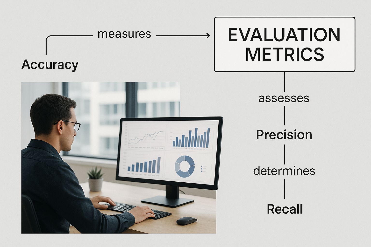
As the graphic shows, a truly robust evaluation strategy isn't about finding one magic number. It's about combining multiple metrics that are tailored to the specific problem you're trying to solve.
Striking a Balance with F1-Score and Specificity
So, how do you manage this trade-off in practice? That’s where the F1-Score comes in. It’s the harmonic mean of Precision and Recall, blending them into a single score. A model only gets a high F1-Score if both its precision and recall are strong, making it a fantastic go-to metric when you need a solid balance between the two.
Another vital metric, especially for any kind of screening tool, is Specificity. It measures how well the model identifies the "negatives"—the healthy cases. It answers the question, "Of all the truly healthy patients, how many did our model correctly identify as clear?" Specificity is the flip side of recall and is directly tied to the false positive rate. A screening AI needs high specificity to be practical; otherwise, it would constantly cry wolf, burying doctors in false alarms.
In the end, choosing the right set of metrics always comes back to the context of the problem and the real-world consequences of your model's inevitable mistakes.
To make these concepts more concrete, let's look at a hypothetical scenario. Imagine an AI model screens 1000 scans for a specific disease, and we know the ground truth for each scan. The table below breaks down how each metric would be interpreted in this clinical context.
Classification Metrics Explained with a Medical Imaging Example
| Metric | What It Measures | Importance in Medical Diagnosis |
|---|---|---|
| Accuracy | The overall percentage of correct predictions (both positive and negative). | Can be misleading if the disease is rare. A high score might hide a model's failure to detect actual cases. |
| Precision | Of all the scans flagged as "disease present," the percentage that were actually positive. | Crucial for minimizing false alarms. High precision reduces unnecessary patient anxiety and costly follow-up procedures. |
| Recall (Sensitivity) | Of all the scans that actually had the disease, the percentage the model successfully identified. | The most critical metric for not missing disease. High recall is vital to ensure patients get timely treatment. |
| F1-Score | The harmonic mean of Precision and Recall, providing a single score that balances both. | Useful when you need a model that is both reliable in its positive predictions and thorough in finding all cases. |
| Specificity | Of all the scans that were actually disease-free, the percentage the model correctly identified. | Essential for screening programs. High specificity ensures that healthy individuals are not constantly flagged for follow-up. |
As you can see, each metric shines a spotlight on a different aspect of the model's behavior. A successful medical AI is never judged by one number alone but by a thoughtful evaluation across a spectrum of these critical measures.
Evaluating Regression and Segmentation Models
While metrics like precision and recall are the bread and butter for classification tasks, the world of medical AI is far bigger than just sorting scans into "cancer" or "no cancer" piles. Many of the most critical jobs involve predicting a specific number or drawing a precise shape. For these challenges, we need a different set of tools in our machine learning model evaluation toolkit.
Let's dive into two other common tasks in medical imaging: regression and segmentation. Each has its own definition of what "good performance" looks like, and understanding these differences is what separates a model that's just technically correct from one that's genuinely useful in a clinic.

Measuring Predictions with Regression Metrics
Regression models are all about predicting continuous values. Think of an AI that estimates a tumor's volume in cubic millimeters, predicts how many days a patient will need to recover, or forecasts blood pressure. In these cases, a simple "yes" or "no" doesn't work. The goal is to get as close as possible to the true value.
Imagine you’re trying to guess the weight of a dozen different objects. To see how you did, you wouldn't just count right vs. wrong; you'd measure how far off each guess was. Two of the most common ways to do this are Mean Absolute Error (MAE) and Root Mean Squared Error (RMSE).
-
Mean Absolute Error (MAE): This is the most straightforward approach. It's simply the average of all your errors, ignoring whether you were high or low. If you guessed 5 grams over on one object and 3 grams under on another, your average error is 4 grams. MAE gives you a clear, easy-to-interpret average error in the original units.
-
Root Mean Squared Error (RMSE): This metric gets a little more mathematical, but for good reason. It squares each error before averaging them and then takes the square root of the result. The key effect here is that squaring the errors gives much more weight to big mistakes. A single, wildly inaccurate prediction will blow up your RMSE far more than it would your MAE. This makes RMSE incredibly useful when large errors are particularly dangerous or unacceptable.
Another key player is the R-squared (R²) value. Instead of measuring error, it tells you how much of the variation in the outcome your model can actually explain. An R² of 0.85, for instance, means your model can account for 85% of the variability in the data—a pretty strong indicator that it has a solid grasp on the underlying patterns.
Outlining Success with Segmentation Metrics
Image segmentation is fundamentally a drawing task. The goal is to outline a specific object within an image, like tracing the boundary of a lesion on an MRI or a polyp in a colonoscopy. Here, success isn't about a single number but about spatial accuracy. How well does the AI's predicted shape match the "ground truth" outline drawn by a human expert?
To measure this, we need metrics that quantify the overlap between the model's prediction (the predicted mask) and the expert's label (the true mask).
Think of it like this: you have two overlapping circles. One represents the "true" area of a tumor, and the other is the area predicted by your AI. The best segmentation metrics measure how perfectly those two circles line up.
The two dominant metrics you'll see everywhere in this space are the Dice Coefficient and Intersection over Union (IoU).
-
Intersection over Union (IoU): Also called the Jaccard Index, IoU is incredibly intuitive. You just calculate the area where the two shapes overlap and divide it by the total area they cover when combined (their union). A perfect match gives an IoU of 1, while two shapes that don't touch at all score a 0. It’s a very strict and clear-cut measure of accuracy.
-
Dice Coefficient: This metric is a close cousin to IoU and is extremely popular in the medical imaging community. It’s calculated by doubling the area of the overlap and dividing it by the sum of the areas of both individual shapes. The Dice score often gives slightly more favorable scores than IoU, especially for smaller objects, which can be helpful when you're trying to segment tiny but critical structures.
Both of these metrics give you a score from 0 to 1, where higher is always better. The choice between them often comes down to the specific problem or even the standard practice in a particular research field. But at the end of the day, they both answer the same core question: did our model draw the right shape in the right place?
Essential Techniques for Validating Your Model

Picking the right metrics is only half the battle in machine learning model evaluation. The other half is making sure the numbers you get are actually telling you the truth. A shaky validation strategy can paint a rosy, but dangerously false, picture of your model’s abilities, setting it up for failure when it meets real-world data.
Think of it like this: you wouldn't quiz a student using questions they've already seen the answers to. By that same logic, you can't evaluate a model with the exact same data it learned from. This is where validation techniques come in, forming the bedrock of a trustworthy assessment.
The Basic Train-Test Split
The most straightforward method is the train-test split. You simply carve up your dataset into two pieces: a larger chunk for training the model and a smaller, completely separate one for testing it. A common split is 80% for training and 20% for testing.
This approach is fast and easy to implement, but it has one glaring weakness. What if, just by sheer luck, the 20% you picked for the test set was unusually easy or incredibly difficult? Your results would be skewed, giving you a biased and unreliable snapshot of the model's true performance.
A single train-test split is like giving a student just one practice exam. Their score might be great or terrible, but you have no way of knowing if that one exam was a true representation of their overall knowledge.
K-Fold Cross-Validation for More Robust Results
To get a more stable and reliable performance estimate, we can turn to k-fold cross-validation. This technique is a bit more involved, but it systematically uses your entire dataset for both training and testing, which gives you a more averaged and dependable result.
Here’s the breakdown of how it works:
- Split the Data: First, you divide your entire dataset into 'k' equal-sized segments, often called "folds." A common choice for 'k' is 5 or 10.
- Iterate and Train: Next, you run 'k' rounds of training and testing. In each round, one fold is held out as the test set, while the other k-1 folds are used to train the model.
- Average the Scores: After running through all 'k' rounds, you average the performance scores from each one. This final average score is a much more robust estimate of how well your model will generalize to new, unseen data.
This process ensures that every single data point gets a turn in the test set, smoothing out the random fluctuations that can plague a simple train-test split.
Handling Imbalanced Data with Stratified K-Fold
In medical imaging, perfectly balanced datasets are a luxury. You'll often find that they're heavily imbalanced. For instance, a dataset of chest X-rays might contain 95% healthy scans and only 5% showing a rare disease.
With standard k-fold cross-validation, one of your folds could, by chance, end up with zero examples of the rare disease. This would completely throw off your evaluation.
That's where Stratified K-Fold becomes absolutely essential. It’s a smarter version of k-fold that makes sure each fold has the same percentage of samples for each class as the original dataset. If your whole dataset has a 95/5 split, every single fold will also maintain that 95/5 split, guaranteeing your evaluation is always representative.
The Importance of a Validation Set
When you're building a model, you often need to fiddle with its internal settings, which are known as hyperparameters. To fine-tune these without "contaminating" your final test set, you need to introduce a third data split: the validation set.
Here’s the proper, disciplined workflow:
- Training Set: Used exclusively to teach the model.
- Validation Set: Used to tune hyperparameters and make decisions about the model's architecture.
- Test Set: Kept under lock and key until the very end, used only once for a final, unbiased evaluation.
This three-way split isn't just academic; it was critical in achieving landmark results. In 2012, the AlexNet model hit a top-5 error rate of 15.3% on the ImageNet dataset—a massive leap at the time. By 2015, more advanced validation protocols helped models like ResNet slash that error rate to just 3.57%.
Understanding these principles is vital, even as tools become easier to use. Platforms like no-code AI app builders simplify development, but the core need to properly validate a model's performance never goes away.
Getting the Full Picture with ROC and PR Curves
Metrics like Precision and F1-Score are great for a quick snapshot, but they only tell part of the story. They measure performance at a single, fixed decision point. To truly understand how a model behaves, we need to see how it performs across all possible decision points.
This is where visualizations come in. Two of the most powerful tools in our arsenal are the Receiver Operating Characteristic (ROC) curve and the Precision-Recall (PR) curve. Think of these not as static charts, but as dynamic maps of the trade-offs your model makes with every prediction. Applying good data visualization best practices here is key to pulling out clear, actionable insights.
Understanding the ROC Curve and AUC
The ROC curve is a classic in diagnostics. It charts the True Positive Rate (TPR) against the False Positive Rate (FPR) at every conceivable classification threshold.
Let’s break that down. Most models don't just spit out a hard "yes" or "no." They give a confidence score, say from 0 to 1. The threshold is the line you draw in the sand (e.g., "anything over 0.7 is a positive case"). The ROC curve beautifully illustrates what happens as you slide that line from 0 all the way to 1.
- A model that’s just guessing will produce a straight diagonal line. No better than a coin flip.
- A strong model, however, creates a curve that arches sharply up and to the left. This means it's racking up true positives without accumulating many false alarms.
This curve gives us a single, wonderfully elegant metric: the Area Under the Curve (AUC). It condenses the entire performance curve into one number between 0 and 1. An AUC of 1.0 is the holy grail—a perfect model. An AUC of 0.5 means the model has zero predictive power. It's a fantastic, high-level summary of your model's classification muscle.
A high AUC score shows that your model is fundamentally good at telling the positive and negative classes apart, no matter which specific threshold you end up choosing. It’s a pure measure of separability.
When a PR Curve Tells a Better Story
ROC curves are great, but they have an Achilles' heel: they can paint a deceptively rosy picture when dealing with highly imbalanced datasets. This is the norm in medical imaging, where you might have thousands of healthy scans for every one showing disease.
This is exactly where the Precision-Recall (PR) curve steps into the spotlight. It plots the direct trade-off between Precision and Recall across different thresholds. Since both of these metrics are laser-focused on the positive class, the PR curve gives a much more sober and realistic view when positive cases are needles in a haystack.
How do you read a PR curve?
- A poor model will have a curve that hugs the bottom of the graph.
- A great model will have a curve that pushes toward the top-right corner, showing it can maintain high precision even as it finds more and more positive cases (high recall).
Imagine you're building a cancer detection model where only 1% of scans are malignant. The PR curve is infinitely more useful here. It directly answers the vital clinical question: "If we tune our model to find every last tumor (pushing for higher Recall), how many of our positive flags will turn out to be false alarms (a drop in Precision)?" This makes it an absolutely essential tool for judging models destined for real-world medical use.
Avoiding Common Evaluation Pitfalls
Even with the best metrics and validation techniques, a shaky evaluation process can completely sink your project. It's how you end up with a model that looks incredible in the lab but falls apart the moment it sees real-world data. A solid machine learning model evaluation isn't just about running scripts; it's about being your model's biggest critic, actively trying to break it so you can find its weaknesses before they can cause real harm.
Think of this as a field guide to the most expensive and damaging mistakes in model evaluation. Getting these right is the difference between building a model that's just "accurate" and one that's genuinely trustworthy—especially when patient health is on the line.
The Cardinal Sin of Data Leakage
The most notorious trap is data leakage. This is what happens when information from outside the training set accidentally sneaks into your model during development. It’s the machine learning version of a student getting the answer key before a test. They might get a perfect score, but that score is completely meaningless.
Data leakage can be surprisingly sneaky. A classic example is normalizing or scaling your entire dataset before you split it into training and testing sets. When you do that, information about the test set's data distribution—like its mean or standard deviation—"leaks" into the training process. The model gets an unfair preview of the test data, leading to an inflated performance score that will never hold up in a real clinical setting.
Your test set should be treated like a vault, sealed and untouched until the final, one-time evaluation. Every preprocessing step—from scaling to feature engineering—must be learned on the training data only and then applied to your validation and test sets.
Choosing a Metric That Hides the Truth
Another common blunder is picking a metric that tells a convenient but misleading story. As we’ve covered, accuracy is a terrible choice for imbalanced datasets, where one class vastly outnumbers the other. When you optimize for a single, ill-suited metric, you can hide a model's most dangerous flaws.
Imagine a model built to detect a rare but aggressive cancer. If your only goal is accuracy, the model could learn to just predict "no cancer" for every single patient. It would achieve 99.9% accuracy and be a complete clinical disaster. The real-world cost of that one missed case (a false negative) is catastrophic.
To get this right, always work backward from the clinical problem:
- What's the cost of a false positive? If it’s high (like triggering an unnecessary, invasive biopsy), then Precision is your north star.
- What's the cost of a false negative? If it's dire (like missing a treatable tumor), then Recall becomes non-negotiable.
- Do you need a balance? The F1-Score is your friend here, as it penalizes models that try to game one metric at the expense of the other.
Picking the right metric is about making sure the math you're optimizing for aligns with the real-world outcome you need.
Ignoring the Deployment Environment
A model doesn't live in a sterile lab. Its real-world performance is deeply connected to the environment where it's actually used. A model trained exclusively on high-resolution, perfectly lit images from a brand-new MRI machine might stumble badly when it encounters lower-quality scans from an older machine in a different hospital.
This gap between pristine training data and messy, real-world data is a huge reason why models fail after deployment. Your evaluation process has to anticipate this. Test your model on data from different sources, under varying conditions, and from multiple types of equipment if you can. This is how you build a model that is robust enough to generalize beyond the clean, predictable world of its training set.
Forgetting That Models Get Stale
Finally, a model's performance isn't set in stone. It can, and will, degrade over time. This is a phenomenon known as concept drift, and it happens when the real-world data starts to look different from the data the model was trained on. A hospital might introduce a new type of scanner, patient demographics might shift over a few years, or new disease subtypes could emerge.
A model that was state-of-the-art last year could be dangerously out of sync today. Forgetting to monitor for this is a critical oversight.
Effective machine learning model evaluation doesn't end at launch. It’s a continuous cycle that includes monitoring the model's live performance and having a clear plan to retrain it with fresh data. A truly robust evaluation framework accounts for the entire lifecycle of the model, not just its debut.
Frequently Asked Questions About AI Model Evaluation
Diving into model evaluation often brings up the same handful of questions. Let's tackle some of the most common ones to give you clear, practical answers you can use right away.
What Is the Best Evaluation Metric to Use?
This is the classic question, and the honest answer is: there's no single "best" one. The right metric always depends on your specific goal and what happens in the real world when your model gets something wrong.
Think of it this way:
- For diagnostic screening, where missing a positive case could be disastrous, Recall is your top priority. You want to catch every possible instance of disease, even if it means flagging a few healthy patients for a second look.
- When confirming a diagnosis just before a high-risk surgery, Precision becomes king. Here, a false positive could lead to an unnecessary procedure, so you need to be absolutely certain every positive prediction is correct.
- For more balanced scenarios, or when you need a single number that captures the trade-off, the F1-Score is a solid choice. It gives you a harmonic mean of both precision and recall.
The question isn't "Which metric is the best overall?" but rather, "Which metric actually tells me if my model is succeeding at its specific job?" The context of the problem is everything.
How Does Evaluation Change for Deep Learning Models?
The fundamental metrics don't change, but the evaluation process gets a lot more complex. Deep learning models are incredibly powerful but are often called "black boxes" for a reason—it's tough to see what's happening inside.
Because of this, just looking at performance scores isn't enough. We need to go deeper. Techniques like saliency maps or Class Activation Mapping (CAM) are crucial. They create heatmaps that show us which parts of an image the model "looked at" to make its decision. This helps confirm it’s focusing on actual clinical features and not just some random artifact in the scan.
How Do You Handle Imbalanced Datasets During Evaluation?
Imbalanced data is practically a given in medical imaging—diseases are often rare. Using a metric like standard accuracy on these datasets is a huge mistake; a model can achieve 99% accuracy by simply guessing "no disease" every time.
Instead, you need to use metrics that don't get thrown off by the class imbalance. The Precision-Recall (PR) curve is much more insightful than a standard ROC curve here. For validation, you absolutely must use techniques like Stratified K-Fold Cross-Validation. This method guarantees that each "fold" or slice of your data has the same proportion of positive and negative cases as the complete dataset, giving you a much more trustworthy assessment of your model's performance.
At PYCAD, we live and breathe these challenges every day. We specialize in building and deploying robust AI for medical imaging, managing everything from tricky datasets to rigorous model validation. If you want to ensure your models are not just technically accurate but truly reliable in a clinical setting, see how we can help your project at https://pycad.co.