Preprocessing 3D volumes for tumor segmentation in MONAI

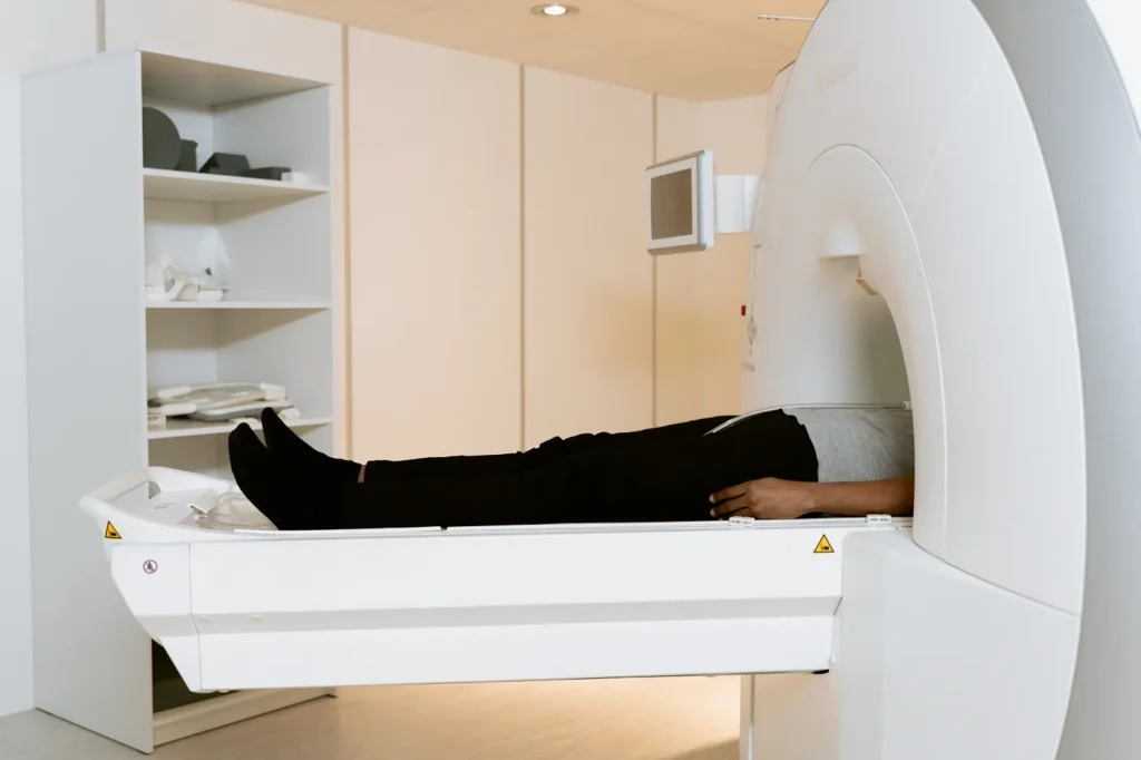
This is MONAI 3D preprocessing for tumor / organ segmentation: load paired NIfTI, resample spacing, window HU, crop empty air, resize, then a Dataset + DataLoader. It is not random flip / rotate / noise — that is 3D volume augmentation in MONAI. It is not how a clinician calculates tumor volume.

The volumes here are CT NIfTI (a stack of slices = one patient). The same compose works on MRI if you change the intensity window. If you still have a DICOM series, convert it first — DICOM to NIfTI. DICOM vs NIfTI: that write-up.

Video of the same 2021 notebook: preprocessing 3D volumes in MONAI.

Install

pip install monai torch torchvision nibabel

Use a venv. AddChanneld below is the 2021 dictionary API; current MONAI uses EnsureChannelFirstd for the same channel dim. Docs: docs.monai.io.

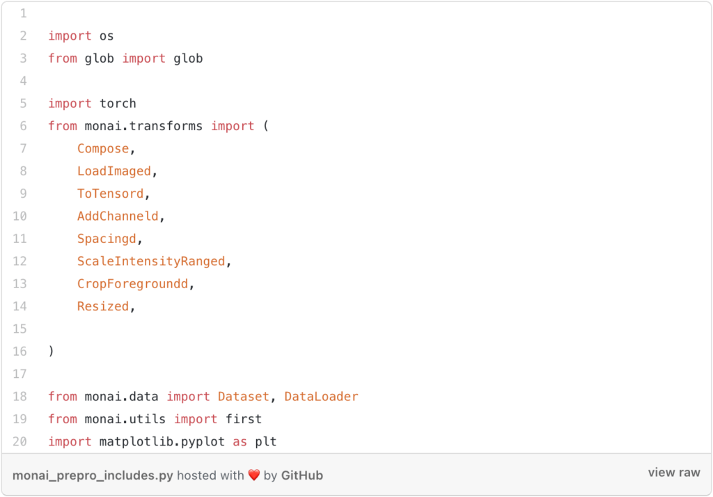
import os
from glob import glob

import torch
from monai.transforms import (
    Compose,
    LoadImaged,
    ToTensord,
    AddChanneld,
    Spacingd,
    ScaleIntensityRanged,
    CropForegroundd,
    Resized,
)
from monai.data import Dataset, DataLoader
from monai.utils import first
import matplotlib.pyplot as plt

Path dictionary

Two ways to load: images and masks as two lists, or one Python list of dicts with image and label keys. The dict is the one you want. Every transform takes a keys= argument, so intensity hits the CT only and spacing hits both.

Four folders: TrainData, TrainLabels, ValData, ValLabels. Pair by sorted filename.

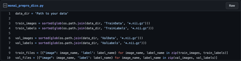
data_dir = 'D:/3_Stage/ALL_THE_DATA/fixed_data_03_august/all_together'

train_images = sorted(glob(os.path.join(data_dir, 'TrainData', '*.nii.gz')))
train_labels = sorted(glob(os.path.join(data_dir, 'TrainLabels', '*.nii.gz')))

val_images = sorted(glob(os.path.join(data_dir, 'ValData', '*.nii.gz')))
val_labels = sorted(glob(os.path.join(data_dir, 'ValLabels', '*.nii.gz')))

train_files = [{"image": image_name, 'label': label_name} for image_name, label_name in zip(train_images, train_labels)]
val_files = [{"image": image_name, 'label': label_name} for image_name, label_name in zip(val_images, val_labels)]

train_files[0] is one patient: path to the volume and path to the mask.

The transforms

Compose stacks dictionary transforms. Required: LoadImaged (read the NIfTI) and ToTensord (torch, so training can start). The rest is what actually makes CT volumes trainable.

Transform	Keys	What it does here
LoadImaged	image, label	Read .nii / .nii.gz.
AddChanneld	image, label	Insert the channel dim the network expects (2021 name).
Spacingd	image, label	Resample to pixdim=(1.5, 1.5, 2) mm. Image bilinear, label nearest (or default if you omit mode).
ScaleIntensityRanged	image only	HU window -200..200 → 0..1, clip=True. Do not scale the mask.
CropForegroundd	image, label	Drop empty air. source_key='image'.
Resized	image, label	spatial_size=[128, 128, 128]. Needed after crop, or every patient has a different shape.
ToTensord	image, label	Torch tensors.

The trailing d means dictionary. Drop it if you are not using a dict. keys picks image, label, or both. Intensity is image-only so the 0/1 mask stays 0/1.

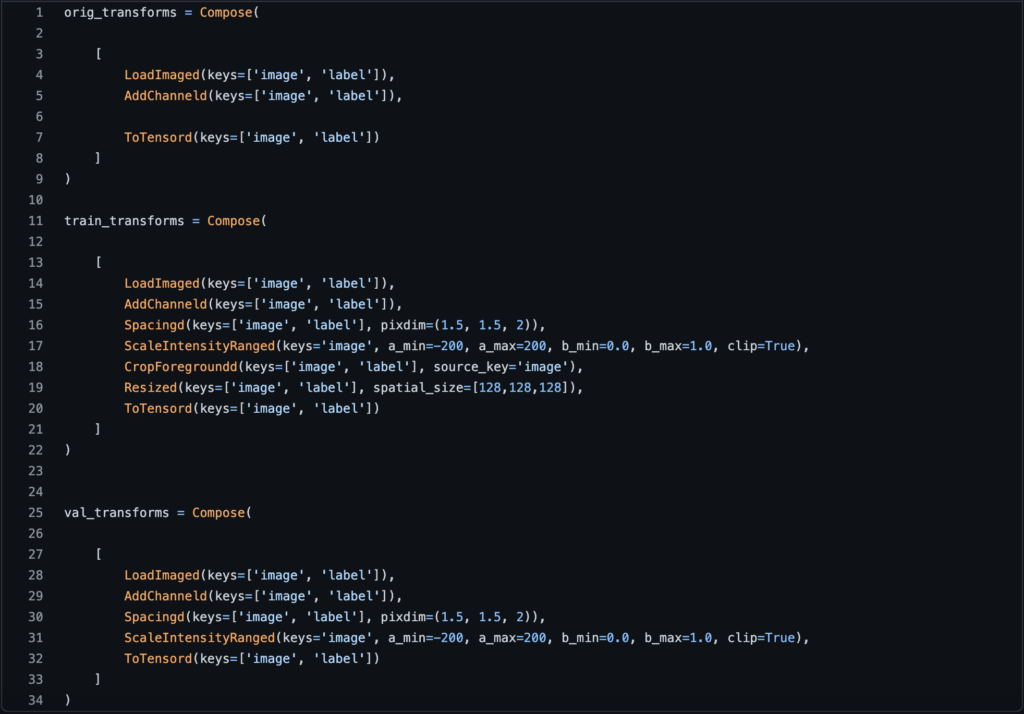
Three composes from the notebook: orig_ (load only, for the before plot), train_ (full stack), val_ (spacing + window, no crop / resize — that is how the 2021 file was written).

orig_transforms = Compose(
    [
        LoadImaged(keys=['image', 'label']),
        AddChanneld(keys=['image', 'label']),
        ToTensord(keys=['image', 'label'])
    ]
)

train_transforms = Compose(
    [
        LoadImaged(keys=['image', 'label']),
        AddChanneld(keys=['image', 'label']),
        Spacingd(keys=['image', 'label'], pixdim=(1.5, 1.5, 2)),
        ScaleIntensityRanged(keys='image', a_min=-200, a_max=200, b_min=0.0, b_max=1.0, clip=True),
        CropForegroundd(keys=['image', 'label'], source_key='image'),
        Resized(keys=['image', 'label'], spatial_size=[128,128,128]),
        ToTensord(keys=['image', 'label'])
    ]
)

val_transforms = Compose(
    [
        LoadImaged(keys=['image', 'label']),
        AddChanneld(keys=['image', 'label']),
        Spacingd(keys=['image', 'label'], pixdim=(1.5, 1.5, 2)),
        ScaleIntensityRanged(keys='image', a_min=-200, a_max=200, b_min=0.0, b_max=1.0, clip=True),
        ToTensord(keys=['image', 'label'])
    ]
)

DataLoader

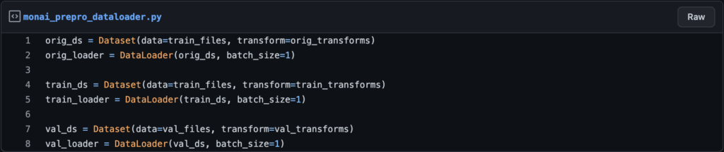
Dataset binds the file list to a compose. DataLoader batches it (here batch_size=1). Two of each if you have train and val.

orig_ds = Dataset(data=train_files, transform=orig_transforms)
orig_loader = DataLoader(orig_ds, batch_size=1)

train_ds = Dataset(data=train_files, transform=train_transforms)
train_loader = DataLoader(train_ds, batch_size=1)

val_ds = Dataset(data=val_files, transform=val_transforms)
val_loader = DataLoader(val_ds, batch_size=1)

Plot one patient

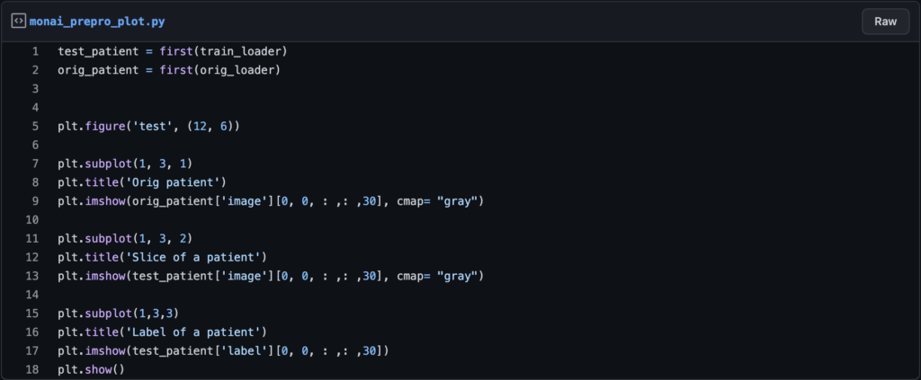
first(loader) is the first batch. Slice index 30 in the notebook.

test_patient = first(train_loader)
orig_patient = first(orig_loader)

plt.figure('test', (12, 6))

plt.subplot(1, 3, 1)
plt.title('Orig patient')
plt.imshow(orig_patient['image'][0, 0, :, :, 30], cmap="gray")

plt.subplot(1, 3, 2)
plt.title('Slice of a patient')
plt.imshow(test_patient['image'][0, 0, :, :, 30], cmap="gray")

plt.subplot(1, 3, 3)
plt.title('Label of a patient')
plt.imshow(test_patient['label'][0, 0, :, :, 30])
plt.show()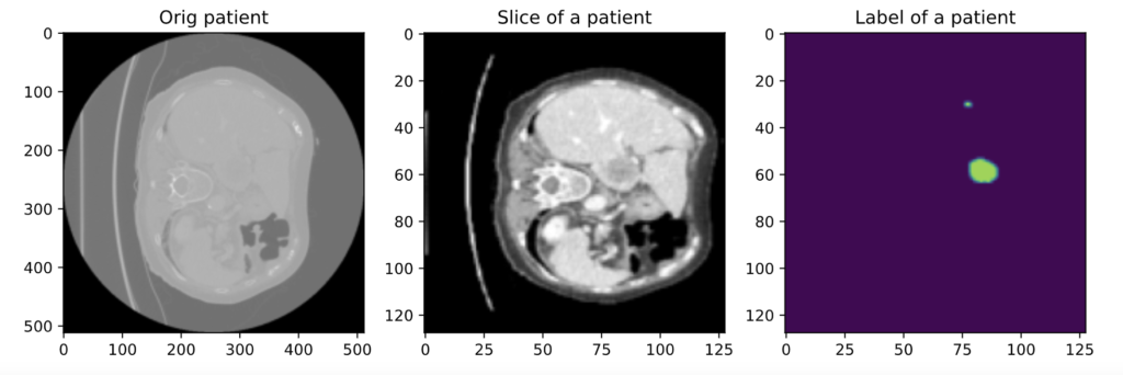

Left is the raw slice. Middle is after spacing / window / crop / resize. Right is the mask. Random affine, rotate, and Gaussian noise are the next step — 3D volume augmentation in MONAI — not this page.

Notebook: amine0110/preporcess-volume-medical-imaging.

PYCAD builds custom segmentation pipelines and web DICOM viewers when the mask has to live next to the series in an app. Case studies.