
Accelerated MRI leaves most of k-space unacquired, so a reconstruction pipeline has to invent the missing coefficients from the ones the scanner kept. Diffusion and flow models can do that well, but they often need hundreds of network evaluations per slice. A team at Bilkent University and Bogazici University (M. Usama Mirza, Esin O. Isik and Tolga Cukur) posted arXiv:2610.13095 on 9 October 2026 with FLEX-MRI. It recovers multi-coil brain MRI in a small number of finite transitions, explores alternate k-space paths with a cheap random perturbation, then snaps each step back to the acquired measurements. The GitHub repository has training and evaluation code. It does not ship pretrained weights.
What goes in and what comes out
The input is undersampled multi-coil complex k-space from a 2D Cartesian brain acquisition, at acceleration rates R = 4, 6 or 8 in the paper’s tests. The output is a reconstructed magnitude image for that cross-section. The authors train and test on high-field fastMRI and low-field M4Raw, covering T1, T2 and FLAIR contrasts.
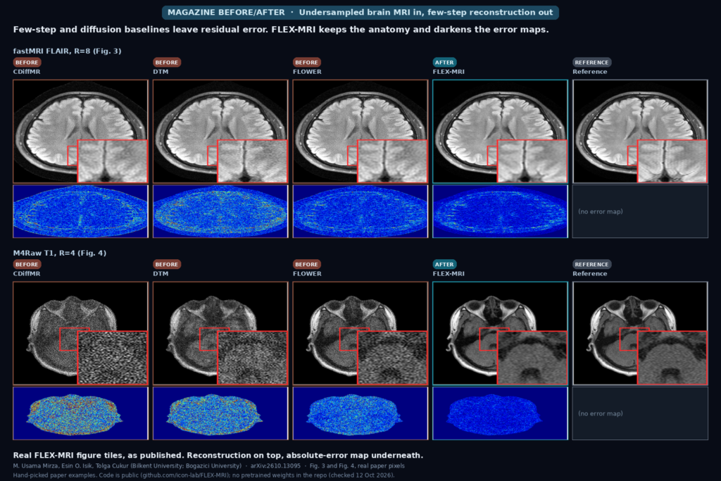
The featured image is built from Fig. 3 and Fig. 4 of the paper, with every tile taken as published and only cropped and resized. The top row is a fastMRI FLAIR slice at R = 8. The bottom row is an M4Raw T1 slice at R = 4. In each row, three baselines sit on the left, FLEX-MRI is in the middle, and the fully sampled reference is on the right. Absolute-error maps sit under every reconstruction except the reference.
How it works
Most generative MRI reconstructors learn small local steps along a long recovery path. FLEX-MRI instead picks a short list of retained states defined by how much k-space support has been filled in, and trains a U-Net predictor to jump across each retained interval in one shot. In the paper’s setting there are J = 10 retained transitions, and the endpoint of the forward process is defined at R = 6.
Training does not lock the loss to one fixed mask. Randomized undersampling masks define the finite-transition targets, and the prediction loss is evaluated across the image without restricting it to the coefficients selected by each individual mask. The authors call this support-relaxed finite-transition learning.
At inference the model does something extra before each jump. It randomly drops or perturbs a subset of the currently estimated k-space coefficients (perturbation rate γj = 0.1 in the reported runs), lets the predictor propose the next image from that perturbed state, then projects the result back onto the acquired measurements with a data-consistency step. The claim is that this stochastic exploration covers the residual ambiguity that a single finite jump cannot resolve, without putting a second generative sampler inside every transition.
What the numbers say
On fastMRI (Table II), FLEX-MRI is best across R = 4 to 8. At R = 8 it reaches 35.8 ± 2.2 dB PSNR and 92.7 ± 5.0% SSIM. Averaged across rates, that is about 2.7 dB and 4.4% SSIM above the diffusion baselines (DDPM, DiffRecon, CDiffMR, FDB), and about 4.6 dB and 11.3% above the few-step flow and transition-matching baselines (FLOWER, UPMRI, DTM).
On noisier low-field M4Raw (Table III), the absolute scores are lower for every method, and FLEX-MRI is still highest: 23.9 / 76.9 at R = 4, 23.5 / 75.1 at R = 6, and 23.2 / 74.3 at R = 8 (PSNR in dB / SSIM in %). Averaged across rates it sits about 4.1 dB and 35.1% SSIM above the diffusion group, and about 2.1 dB and 23.3% above the few-step group.
Models trained on M4Raw and tested on fastMRI without retraining (Table IV) keep most of that gain. FLEX-MRI scores 37.6 / 94.2 at R = 4 and 34.8 / 92.2 at R = 8, which is only about 0.8 dB and 0.4% SSIM under its in-domain fastMRI numbers.
Timing matters for a viewer or batch recon job. On one Nvidia RTX 4090, a single cross-section takes 0.349 s and 1.05 GB for FLEX-MRI (Table V). That sits with the few-step baselines (DTM 0.437 s, FLOWER 0.477 s, UPMRI 0.318 s) and is roughly two orders of magnitude faster than the 1000-step diffusion runs (DDPM 37.12 s, DiffRecon 36.26 s). Peak memory for FLEX-MRI matches the few-step group at 1.05 GB, while the diffusion methods sit between 1.71 and 3.19 GB.
What the pictures show
In the fastMRI FLAIR row, CDiffMR and DTM leave grainy residual texture, and FLOWER is smoother but still shows more error than FLEX-MRI. The FLEX-MRI error map is mostly dark, and the zoomed cortical inset tracks the reference more closely than the three baselines. FDB, DDPM and DiffRecon are discussed in the paper as quieter but softer on edges. Those columns are not in the featured crop.
In the M4Raw T1 row the gap is louder. CDiffMR and DTM show heavy pixelation and bright error maps. FLOWER cleans some of that up but still leaves residual structure. FLEX-MRI’s reconstruction is closer to the reference and its error map is the darkest of the compared panels. These are the authors’ selected examples at one acceleration each, so they illustrate failure modes rather than average cases.
Where it falls short
The experiments are supervised reconstructions of 2D Cartesian multi-coil slices. The authors list non-Cartesian sampling, volumetric reconstruction, and broader scanner and protocol variation as open tests. They also say reference-image metrics alone cannot settle diagnostic usefulness, and that radiological evaluation is still needed.
The ablation on fastMRI at R = 8 (Table VI) shows that turning off stochastic exploration or switching to a support-restricted loss drops PSNR and SSIM. Perturbing the training inputs on top of the proposed setup does not help further. The number of retained transitions also matters: quality peaks at J = 10 and falls for both fewer and many more steps (Fig. 5). At J = 2, PSNR and SSIM are 1.7 dB and 1.1% lower than at J = 10. At J = 1000 they are 2.3 dB and 7.8% lower. Inference cost scales roughly with J, so the authors keep the intermediate setting.
Because each run can explore a different k-space path, repeated reconstructions from the same measurements could in principle map uncertainty. The paper only sketches that idea. It does not report a clinician reader study.
Code, weights, and data
The paper points to github.com/icon-lab/FLEX-MRI. On 12 October 2026 that repository held a full PyTorch stack: utils/finite_transition.py (the FlexMRI class), training and sampling scripts, ESPIRiT coil-map caching, and an evaluation script against M4Raw’s reconstruction_rss. The license is MIT. There were no GitHub Releases and no pretrained .pt checkpoints in the tree. The README expects you to download M4Raw, precompute coil maps, and train with train.sh (125,000 iterations in the documented recipe).
The public datasets are fastMRI and M4Raw. Competing methods in the tables include LORAKS, rGAN, DDPM, DiffRecon, CDiffMR, FDB, DTM, FLOWER and UPMRI, all run on the same splits and undersampling patterns.
How we would wire it into a viewer
For a DICOM viewer or recon service we would treat FLEX-MRI as an accelerated reconstruction option next to zero-filling and whatever clinical recon the scanner already provides. Store the reconstructed series as machine-generated, with the model name, J, γ, acceleration and coil-map method in the series description. Keep the acquired k-space or the vendor recon as the primary reading series until a site validates the model on its own protocols.
Before trying it on our own studies we would check four things: whether a checkpoint trained on M4Raw or fastMRI transfers to our field strength and coil geometry, how it behaves on non-Cartesian or 3D acquisitions the paper did not test, whether repeated stochastic runs disagree in ways a reader would notice, and whether 0.35 s per slice still holds once the full volume and coil-map prep are included. The training code is public, so the missing piece is a released weight file and a local validation set. For related accelerated MRI work on this site, see our post on cardiac MRI reconstruction with a frozen pretrained vision encoder.
Sources
- Mirza, M. U., Isik, E. O., Cukur, T. Stochastic Finite-Transition Learning and Exploration for Accelerated MRI Reconstruction. arXiv:2610.13095, 2026. https://arxiv.org/abs/2610.13095. PDF: https://arxiv.org/pdf/2610.13095.
- Project repository (code present, no pretrained weights, checked 12 October 2026): https://github.com/icon-lab/FLEX-MRI.
- Zbontar et al., fastMRI, arXiv:1811.08839. Lyu et al., M4Raw, Scientific Data 10, 2023.
- Featured image: Fig. 3 (fastMRI FLAIR, R = 8) and Fig. 4 (M4Raw T1, R = 4) of arXiv:2610.13095, as published.