In this article, I will talk about how to create a simple deep learning model for linear regression.
Introduction
As we know, deep learning has become a very important branch in the world and in all fields because they have found that it gives good results and with an accuracy close to 100%, the only problem with these networks is that to implement them we need to gather data (we are talking about thousands and more) because there are cases where we can’t always find the data to do the learning.
Generally, if we want to implement a deep learning model, we have to go through three steps: training, validation, and testing, but sometimes we can leave the validation step.
In this tutorial, we will try to familiarize ourselves with the ‘Keras library of deep learning and to know the role of each function. At first, we will try to make a simple linear regression, and then we will make a classifier of the images.
Installation of the tools
In order to make a program of deep learning, it is necessary first to install some tools or we can say libraries, so the steps are the following ones.
You need a text editor, to write the program, in my case I will use visual studio code in I have to install the libraries with the following way:
keras → to install keras just type the command ‘pip install keras’
numpy → same thing ‘pip install numpy’ for vector manipulation
matplotlib → ‘pip install matplotlib’ for plotting points and lines.
But in case you use anaconda for example the installation of libraries it won’t be like that, you have to select them.
So after installing the tools, we can start our examples using the same libraries.
linear regression
Explanation
Linear regression consists of finding a function or a line in our case that we call the optimal line that passes through most of the points or samples we have, and after having the equation of this line it will be easy to determine the image of any point.
The equation of a simple line → Y = aX + b
So the role of our learning is to find the values of a and b which are the weights of the model and of course after having the weights a and b we can easily determine the values of the Y for the X’s in the input.
Importing the libraries
So as with any program in python you always have to import the libraries before using them, so for our example, we will need the three libraries: Keras, numpy, and matplotlib.
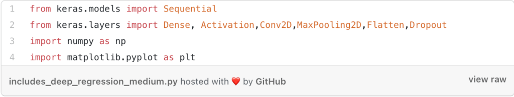
→ We’re going to use a sequential model: the role of the sequential model is to let us build our model by ourselves, i.e. layer by layer (the opposite and transfer learning: using pre-trained models)
→ And then we imported the different functions that we will talk about next.
→ Of course, we have to import numpy for the generation of the samples and matplotlib for the plotting at the end.
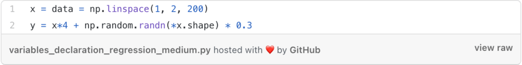
Creating the data
For this example we need to create the input and output data for the training, so we created vectors with random values using numpy.
Creation of the sequential network
As we said, our case is very easy and the network consists of a single DENS tick and this layer contains a single neuron with the activation function ‘linear’, the role of this function is to create an output proportional to the input by multiplying the input by the network weights.
The neuron will be like this:
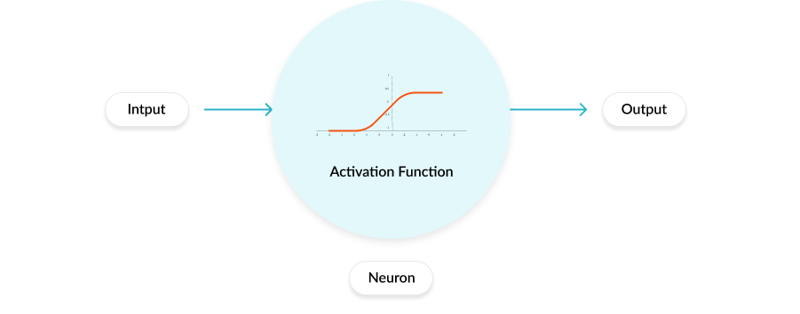
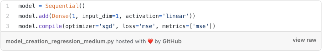
So for the parameters of the add function that will add the DENS layer, we have the first parameter ‘1’ to say that we have only one neuron, the second parameter to say that the dimensions of the input are 1, and of course the activation function that we talked about.
And for the function ‘compile’ we also have parameters, for the optimizer we chose the method of the descent of gradient, and for the function loss which is going to calculate the error so in this case, we used the function ‘mse’ for ‘mean squared error’ this function consists simply in calculating the square of the difference between the real value and the predicted value.
Displaying initial weights
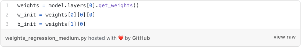
So as said, the goal of this program is to find the values of a and b for the optimal line, so here the a and b are the two weights w_init and b_init.
The learning process
After configuring all the parameters, now you just have to start the training with the fit function.

So in this function, we can see that there are parameters that we haven’t already talked about, it’s the batch_size parameter that will control the number of samples per iteration that we will take during the training and the epochs parameter to fix the number of iterations that we will do for the training.
The test
So after the training, we have to test the model which means we have to use the a and b we found to predict the outputs of other samples.
First, we will display the values of the weights after learning, and then we will make the prediction part.
The values of the weights after learning:
w_after = 3.7 (but it varies in each execution because we have the randn function but it will always be between 3.5 and 4 because if we notice very well, the value of a is already given at the beginning of the program in the definition of Y we had (4 x …) ).
b_after = 0.56 (also varies)
Now we have to make an example of prediction to see if the model has learned well or not, so we will take the simplest case is to take the input vector entirely and apply the weights we have obtained so normally we should have the optimal line between all the input samples.
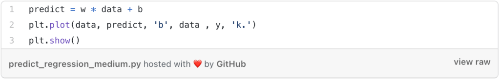
So that was the program that helps us to do a linear regression, so we get the following results:
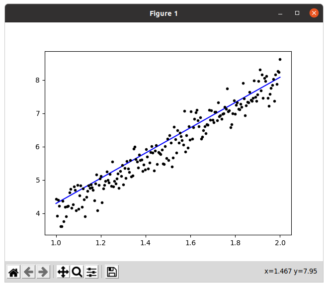
So we can see that the line passes through the middle of the points, which means that it touches the maximum of the points and we can always optimize it by changing the number of iterations, if we increase the number of iterations the result can be optimized more and more and even if we increase the batch_size it also optimizes the result.
If we take the values of the loss function we find the following results:
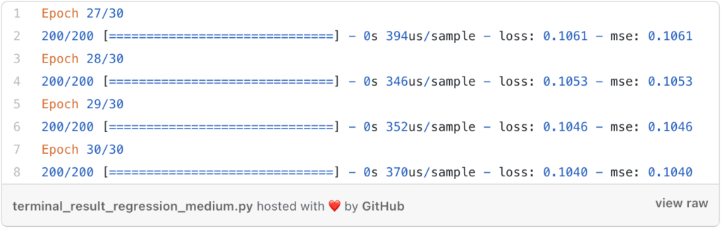
We can notice that the value of the error decreases after each iteration when this is what we want so the learning works very well and also we see that the error is very small which means that the precision is important.
Find a sponsor for your web site. Get paid for your great content. shareasale.com.