
Anyone who has pushed a glioma case through a standard brain pipeline knows how it goes. Skull stripping eats into the tumor or leaves a chunk of it outside the mask. Atlas registration bends the surrounding anatomy out of shape trying to match a mass the atlas has never seen. FreeSurfer-style parcellation either fails outright or labels lesion tissue as white matter or cortex. These tools were built and trained on brains without large holes and lumps in them, and they behave accordingly.
One practical workaround is to give those tools a copy of the scan in which the tumor region has been replaced by tissue that looks like a healthy brain, run the pipeline on that copy, and carry the resulting transforms and labels back to the original. That is what the BraTS inpainting task asks for, and a new paper from the Medical University of Graz is a reproducible entry in it.
Arnela Hadzic, Franz Thaler, Simon Johannes Joham, and Martin Urschler posted arXiv:2610.08983 on 6 October 2026. Their method takes a 3D T1-weighted brain MRI and a binary mask, and fills the masked region with synthetic healthy-looking tissue, one axial slice at a time but with the slices above and below in view. The code, the training split, and a pretrained checkpoint are on GitHub.
What goes in and what comes out
The input is a native T1 volume (t1n in BraTS naming) with the region to fill already set to zero, plus the mask that marks that region. In the challenge data the volumes are 240 x 240 x 155 at 1 mm isotropic, skull-stripped and co-registered as BraTS cases always are. The method crops them to 208 x 208 x 144 and scales intensities to the range -1 to 1, then reverses both steps at the end so the output lands back on the original grid.
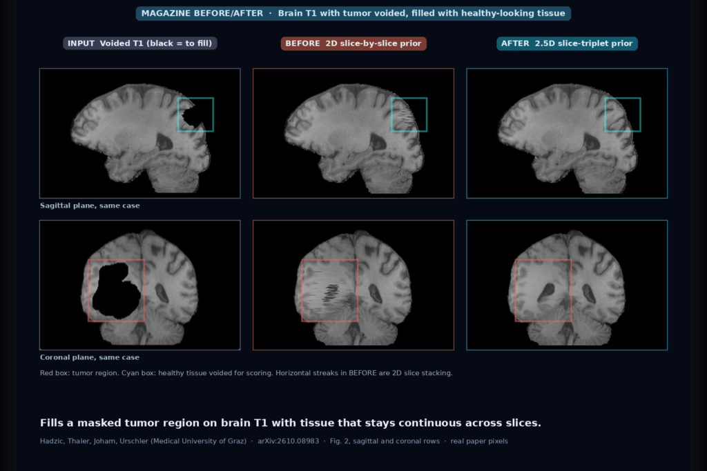
The output is the same T1 volume with the masked voxels replaced. Voxels outside the mask stay as they were. The featured image is Fig. 2 of the paper. In the left column, the black areas are what the model has to fill: a large region around the tumor (red box) and a smaller patch of healthy cortex that the challenge organisers blacked out on purpose (cyan box), because only healthy tissue has a ground truth to score against. The middle column is a 2D baseline that fills each axial slice on its own. The right column is the authors’ 2.5D version.
In the axial plane both look reasonable. The difference shows when you scroll the other way. In the sagittal and coronal views, the 2D fill is a stack of horizontal stripes, because every axial slice made its own guess. The 2.5D fill is continuous through the volume, and in the coronal row it draws a ventricle where the other hemisphere has one, at the spot where the 2D version left dark streaks.
How it works
The generative part is flow matching, a close relative of diffusion models. A network learns a velocity field that moves random noise towards realistic images along a straight path, and at inference an ODE solver follows that field for a fixed number of steps. Here the network is a 2D U-Net with three input and three output channels, and those three channels are three neighbouring axial slices. The model therefore learns what a short stack of healthy brain slices looks like.
Two choices make it work for inpainting. The first is how the prior is trained. BraTS scans all contain tumors, so there is no large set of healthy brains in the same format. The authors train on the challenge scans anyway and switch off the loss inside the tumor mask. Gradients only come from healthy pixels, so the model learns healthy anatomy from the healthy parts of sick brains. It is trained to generate whole slice triplets unconditionally and never sees a hole-filling example.
The second is how the mask is enforced at inference. They use Restora-Flow, a mask-guided sampler that the same group published at WACV 2026. At every solver step, voxels outside the mask are overwritten with a suitably noised copy of the real image, and only the voxels inside the mask are left to the model. A trajectory correction step then nudges the sample back towards the learned distribution so the seam between real and generated tissue does not show. Because the fill comes from the sampler and not from training, the same model handles any mask shape. The authors call this zero-shot inpainting.
To cover a full volume they walk along the superior-inferior axis. For each axial slice that needs filling, the model gets a window of three slices: the one below, which has already been filled in the previous step, the target slice, and the one above. Only the middle slice of the output is kept, and the window moves up by one. Each slice is generated knowing what the model put underneath it, and that is where the continuity comes from.
The last step is optional. Every run starts from different noise, so every run gives a slightly different brain. Averaging ten runs voxel by voxel improves every score, but the authors are open about the cost. An average of ten plausible brains is blurrier than any one of them, so the ensemble looks smoother than a single sample. If you want sharp texture, take one sample.
Data and training
All work is on the BraTS 2026 Inpainting Challenge data: 1,251 training T1 scans, each with the original image, the voided image, the combined mask, and separate masks for the tumor and for the synthetic healthy void. For development the authors split it 90/10 by patient, and the split files are in the repository. The final model was retrained on all 1,251 cases for 10,000 epochs, which took about 100 hours on one NVIDIA A100 with 40 GB.
The official validation set has 219 cases with the ground truth withheld. Scores are computed only inside the synthetic healthy void, since nobody knows what the tissue under a tumor would have looked like.
What the numbers say
On their internal validation split, with the same checkpoint and settings, the 2.5D model reached an SSIM of 0.789 against 0.727 for the 2D baseline, and PSNR went from 18.9 to 20.6 dB. On the official challenge validation set, a single sample scored SSIM 0.793 and the ten-sample average 0.816, with PSNR 21.9 and 22.9 dB.
I would read those as evidence that the slice triplets fix the stacking problem and that the method sits in a reasonable range. The paper does not compare against other challenge entries or against 3D or latent-diffusion inpainting, so it says nothing about where it ranks.
Speed and hardware
With 32 solver steps and one correction step, a single reconstruction took 3 minutes 48 seconds per volume on an RTX 3090 Ti with 24 GB, for an average of 97 masked slices. The ten-sample ensemble, run in parallel, took about 24 minutes, roughly 36% faster than running the ten samples one after another. The authors found that quality levels off at around 32 steps, so there is not much to gain from going higher.
For a clinic this is a background job. Four minutes per case on a consumer-class GPU is easy to schedule on ingest.
Where it falls short
The paper’s own Fig. 4 shows the weak spots. Larger masks get larger flat, homogeneous areas than the matching region in the other hemisphere. Complex structures like the ventricles are sometimes only partly recovered. Far from the edge of the mask, different samples can draw different anatomy, which is expected from a generative model but means a single fill is one guess among many.
A few limits come from the setup. It is T1 only, and it was trained on BraTS-format data that is already skull-stripped, co-registered, and resampled to 1 mm, so a clinical scan needs the same preparation first. If the mask touches the first or last slice of the volume, that slice is skipped, because the three-slice window has nowhere to go. The prior learned healthy tissue from glioma patients, so I would expect some of that tissue to carry mass effect, edema-related signal, or treatment changes the mask did not cover.
The paper also leaves its main use case untested. The stated reason for inpainting is to make registration, brain extraction, and segmentation work better, but this paper measures image similarity in healthy voids, not whether any of those downstream tools improve. Before relying on it, I would want to see atlas registration error or parcellation agreement on inpainted scans compared with the usual lesion-masking approach.
Code, weights, and data
The code is at github.com/imigraz/brats2026-inpainting. It has the training script for the 2.5D prior, scripts for single and ensemble sampling, the 90/10 split files, an example BraTS case folder, and a download script for the 10,000-epoch checkpoint hosted on Google Drive. Inputs and outputs are NIfTI. I did not find a license file in the repository on 8 October 2026, so check with the authors before using it in a product. The README lists the paper as a MICCAI 2026 workshop and challenge contribution. The BraTS training data is available through the challenge under its own terms.
How we would wire it into a viewer
The inpainted volume should never be the image a radiologist reads. It contains tissue that does not exist. In our viewers it would live as a derived series next to the original, marked DERIVED and SECONDARY in Image Type, with a series description that says it is synthetic, and hidden from the default hanging protocol.
The inpainted copy is for the processing pipeline. When a T1 with a tumor segmentation arrives, a worker skull-strips it, resamples it to the 1 mm grid the model expects, runs one inpainting sample, and hands the filled copy to atlas registration or parcellation. The transforms and labels those tools produce get applied back to the original T1, and the tumor mask is laid on top again. If the inpainting does its job, the radiologist sees a sensible parcellation around the real tumor, and the region names in a report come from an atlas fit that the mass did not pull out of shape.
The same derived series is handy for longitudinal comparison and for radiotherapy contouring tools that start from an atlas. In every case I would keep the fill confined to the tumor mask plus a small margin, use a single sample rather than the smoothed average, and test registration and labelling on our own cases before switching it on.
Sources
- Hadzic, A., Thaler, F., Joham, S. J., Urschler, M. Zero-Shot Brain MRI Inpainting with 2.5D Unconditional Flow Priors. arXiv:2610.08983, 2026. https://arxiv.org/abs/2610.08983. PDF: https://arxiv.org/pdf/2610.08983.
- Code and checkpoint: https://github.com/imigraz/brats2026-inpainting.
- Hadzic, A., Thaler, F., Bogensperger, L., Joham, S. J., Urschler, M. Restora-Flow: Mask-Guided Image Restoration with Flow Matching. WACV 2026, pp. 4943 to 4952. https://doi.org/10.1109/WACV61042.2026.00480.
- Kofler, F., et al. The Brain Tumor Segmentation (BraTS) Challenge: Local Synthesis of Healthy Brain Tissue via Inpainting. arXiv:2305.08992, 2023. https://arxiv.org/abs/2305.08992.
- Featured image: Fig. 2 of arXiv:2610.08983, sagittal and coronal rows, voided input, 2D baseline, and 2.5D reconstruction. Box colours are the paper’s.