
Anyone who reads prostate MRI has seen the diffusion series go wrong. The T2 shows a tidy gland, and the b-value images and ADC map next to it show a gland that bulges toward the rectum, loses signal along its back edge, or fades out around a fiducial marker. The cause is the readout. Clinical prostate DWI is almost always single-shot echo-planar imaging (EPI), which is fast but bends the image wherever the magnetic field is uneven, and rectal gas, bowel contents, surgical clips, hip implants, and radiotherapy markers all make it uneven. The same physics keeps routine DWI at about 2 x 2 x 3 mm while the T2 beside it is much finer.
Jingjia Chen, Kun Zhou, Haoyang Pei, Angela Tong, Sherif Elsherif, Luke Ginocchio, Mahesh Bharath Keerthivasan, Qiuting Wen, Hersh Chandarana, and Li Feng (NYU Grossman School of Medicine, Siemens, and Indiana University) describe another way in arXiv:2610.05426, posted 4 October 2026. PROPELLER-DWI pairs a spin-echo based PROPELLER readout, which does not build up field errors the way EPI does, with a self-supervised network that reconstructs and denoises the result. In 25 volunteers and 4 patients on a 3T scanner, it kept the prostate’s shape where EPI warped it, at in-plane resolutions down to 1.25 mm.
What goes in and what comes out
The input is raw multicoil k-space from a prototype sequence on a 3T Siemens MAGNETOM Prisma, acquired at b = 50 and b = 1000 s/mm2 along three diffusion directions. The output is what a reader already expects from a prostate exam: trace-weighted b = 50 and b = 1000 images and an ADC map.
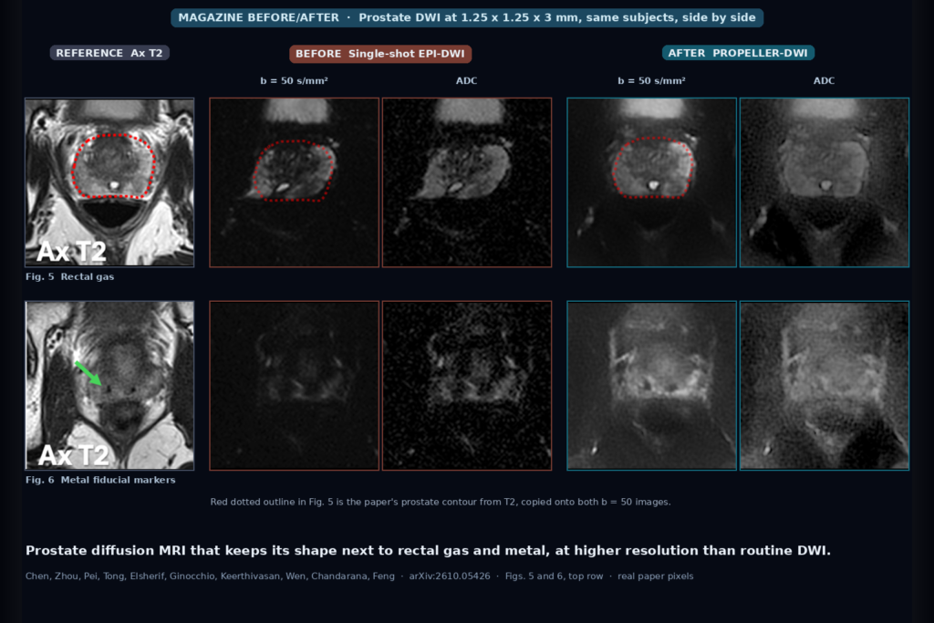
The featured image takes the top row of the paper’s Figs. 5 and 6, where both sequences ran at 1.25 x 1.25 x 3 mm. In Fig. 5, a volunteer with a lot of rectal gas, the red dotted line is the prostate outline from the T2, copied onto both b = 50 images. The EPI gland pushes out of that outline toward the rectum. The PROPELLER gland sits inside it. In Fig. 6, a subject with metallic fiducial markers left from prostate radiotherapy, the EPI b = 50 image at this resolution is mostly signal loss and its ADC map is speckle, while PROPELLER keeps the gland readable on both.
The fairer comparison is the bottom row of those figures, where EPI runs at the clinical protocol (2.0 x 2.0 mm, purple box). EPI looks much better there and still shows distortion and signal loss next to the gas and the metal. At routine resolution EPI is often fine. The gap opens in hard anatomy and at higher resolution.
How the acquisition works
Each shot starts with a conventional pulsed-gradient spin-echo diffusion preparation. A train of refocusing pulses follows, and around each one the sequence reads several gradient echoes (a GRASE readout). Each echo group fills one blade, a narrow strip of k-space through the centre, and every shot rotates the blade pattern by a golden-angle step so the strips do not repeat.
The refocusing pulses remove the distortion. In EPI, each phase-encoding line is read a little later than the one before, so field errors add up into a shift along one direction. Spin echoes reset that error on every echo. Gradient echoes buy speed at the price of some field sensitivity, so the authors tested 1 to 9 per spin echo and settled on 6, with 14 spin echoes per repetition, 28 phase-encoding lines per blade with 2-fold GRAPPA, and an 18.5 degree rotation between shots.
Tiny patient motion during the diffusion gradients scrambles phase and breaks a spin-echo train. The sequence handles this with a phase-insensitive preparation that throws away the unstable half of the signal. That costs SNR, and the network pays it back.
How the reconstruction works
There is no clean, fully sampled prostate DWI to train against, so the network learns from the acquired data. Blade data are phase-corrected one blade at a time and split at random into two disjoint subsets. The network reconstructs an image from one subset and is scored on how well it predicts the other. At inference it sees all the data.
The model is an unrolled variational network with 12 cascades, plus a small U-Net for coil sensitivity maps. Five training rounds each held out 5 subjects plus one common subject and trained on the other 19, so every volunteer was reconstructed by a model that never saw them. Inference took 9.9 seconds per case at 1.8 mm, 14.3 at 1.4 mm, and 16.2 at 1.25 mm on an NVIDIA A100. The five models gave nearly the same images on the common subject (SSIM 0.967 to 0.985 at b = 50, 0.948 to 0.976 at b = 1000). In Fig. 4 the learned reconstruction is cleaner than plain NUFFT and than MPPCA denoising, and the gap grows at 1.25 mm.
What they tested
In the NIST/QIBA diffusion phantom, EPI at 1 x 1 mm warped badly next to a metal bolt and an air bubble, and EPI at 2 x 2 mm warped less. PROPELLER at 1 x 1 mm kept the shapes at a similar scan time of about 5 minutes, with slightly lower apparent SNR, and its ADC values matched the phantom’s reference values.
The in vivo cohort was 25 male volunteers (mean age 41.9) scanned with both sequences at three settings, from roughly clinical (EPI 2.0 mm, PROPELLER 1.8 mm) to 1.4 mm and 1.25 mm, all with 3 mm slices. Four patients (mean age 69.2) got PROPELLER at 1.25 mm as an add-on to their clinical exam. Two had PI-RADS 3 lesions, and lesion position and ADC appearance matched the clinical EPI. The full PROPELLER protocol took 6 min 50 s.
What the radiologists said
Two fellowship-trained body radiologists scored the volunteer images side by side in random left and right order. On geometric fidelity, judged against the T2, PROPELLER scored significantly higher than EPI at all three resolutions. On artifacts it scored significantly higher for every image type and resolution. Overall quality and sharpness favoured PROPELLER in most comparisons, with no significant difference for low-resolution b = 1000 images and high-resolution ADC maps.
Preference followed distortion. When EPI was badly distorted, readers chose PROPELLER significantly more often. In the middle band of EPI fidelity scores (2.5 to 3.5) there was no significant preference. Agreement between the two readers was modest, with weighted kappa of 0.06 to 0.22 for image quality and 0.38 for geometric fidelity, so I would read these results as a direction backed by the figures rather than as precise effect sizes.
What happens to ADC
As someone who builds measurement tools, I care most about this result. Tissue ADC should not depend on voxel size. With EPI it did. ADC in the peripheral and transition zones fell as resolution increased, significantly in both. The authors blame lower SNR, longer echo time, and signal voids at high resolution, which bias ADC downward. PROPELLER ADC stayed steady across the three settings. It ran slightly higher than low-resolution EPI, which the authors think may come from motion between shots mimicking extra diffusion.
Shorter scans
6 min 50 s is long next to the reduced-FOV EPI (ZOOMit) the authors’ site uses for hard cases, which takes 6 min 38 s. Reconstructing the 1.25 mm data retrospectively from fewer shots gave equivalent scan times of 4 min 30 s and 2 min 29 s. In Fig. 10 both stay close to the full scan, with more noise as shots drop and small ADC differences. That is one representative case and a retrospective subsample, so a prospectively shortened protocol still needs testing.
Where it falls short
SNR is still the main limit at b = 1000 and 1.25 mm, and the phase-insensitive preparation discards about half the signal by design. The highest b-value acquired was 1000 s/mm2, while PI-RADS v2.1 asks for a high b-value of at least 1400 s/mm2, acquired or calculated.
The comparison is mostly against single-shot EPI. There is no systematic comparison with reduced-FOV or multi-shot EPI, which many sites already use for difficult cases; one supporting figure shows ZOOMit reducing a metal artifact that PROPELLER handled better, in one subject. Centric echo ordering adds some T2 blurring within each blade, and peripheral nerve stimulation and patient comfort with this readout have not been studied. The cohort is mostly younger healthy volunteers, the patient arm is four people, and the readers scored image quality, not cancer detection. The authors say larger studies with PI-RADS reads and histopathology are needed.
Code and data
Nothing is released. The paper has no code or data availability statement, and I could not find a public repository for the sequence or the reconstruction. The sequence is a Siemens prototype with Siemens co-authors, so the realistic path to a clinic runs through the vendor or a research agreement. The same NYU group maintains the public fastMRI Prostate raw data and reconstruction code for standard prostate T2 and DWI, which does not include PROPELLER-DWI.
What it means for a viewer or clinic workflow
PROPELLER-DWI arrives as a scanner sequence plus a reconstruction step, so the viewer work is downstream. Three things change if a site adopts it.
T2 and DWI start to line up. ADC overlays on T2, lesion contours drawn on T2 and checked on ADC, and DWI-defined targets for MR-ultrasound fusion biopsy or an MR-Linac boost all assume the two series share geometry. With EPI, tools hide the mismatch with deformable registration or the reader corrects it by eye. With PROPELLER a plain linked cursor should be enough, and I would add that check to the hanging protocol with the T2 contour shown on the DWI.
ADC tools need the series context. EPI values move with resolution and PROPELLER values sit a bit higher, so anything that stores ADC thresholds, trends ADC across visits, or feeds a model trained on EPI should record which sequence and voxel size produced the map.
Reconstruction moves off the console. At 10 to 16 seconds per case on an A100, it fits a recon server that pulls raw data and pushes DICOM back to PACS, with the series marked as derived and the model version in the header. If we were building this, the first test would be the paper’s own: EPI and PROPELLER side by side with the T2 on a site’s hardest cases, rectal gas, hip replacements, and post-radiotherapy prostates with markers, and the radiologists deciding which one they read from.
Sources
- Chen, J., Zhou, K., Pei, H., Tong, A., Elsherif, S., Ginocchio, L., Keerthivasan, M. B., Wen, Q., Chandarana, H., Feng, L. Distortion-Free High-Resolution PROPELLER-DWI: Technical Advances and Initial Demonstration for the Prostate. arXiv:2610.05426, 2026. https://arxiv.org/abs/2610.05426. PDF: https://arxiv.org/pdf/2610.05426.
- fastMRI Prostate dataset and reconstruction code (CAI2R, NYU): https://github.com/cai2r/fastMRI_prostate.
- PI-RADS v2.1 (American College of Radiology): https://www.acr.org/Clinical-Resources/Clinical-Tools-and-Reference/Reporting-and-Data-Systems/PI-RADS.
- Featured image: top rows (1.25 x 1.25 x 3 mm) of Figs. 5 and 6 of arXiv:2610.05426, showing the axial T2w reference, EPI-DWI and PROPELLER-DWI b = 50 images, and ADC maps. Red dotted contour and green arrow are the paper’s.