
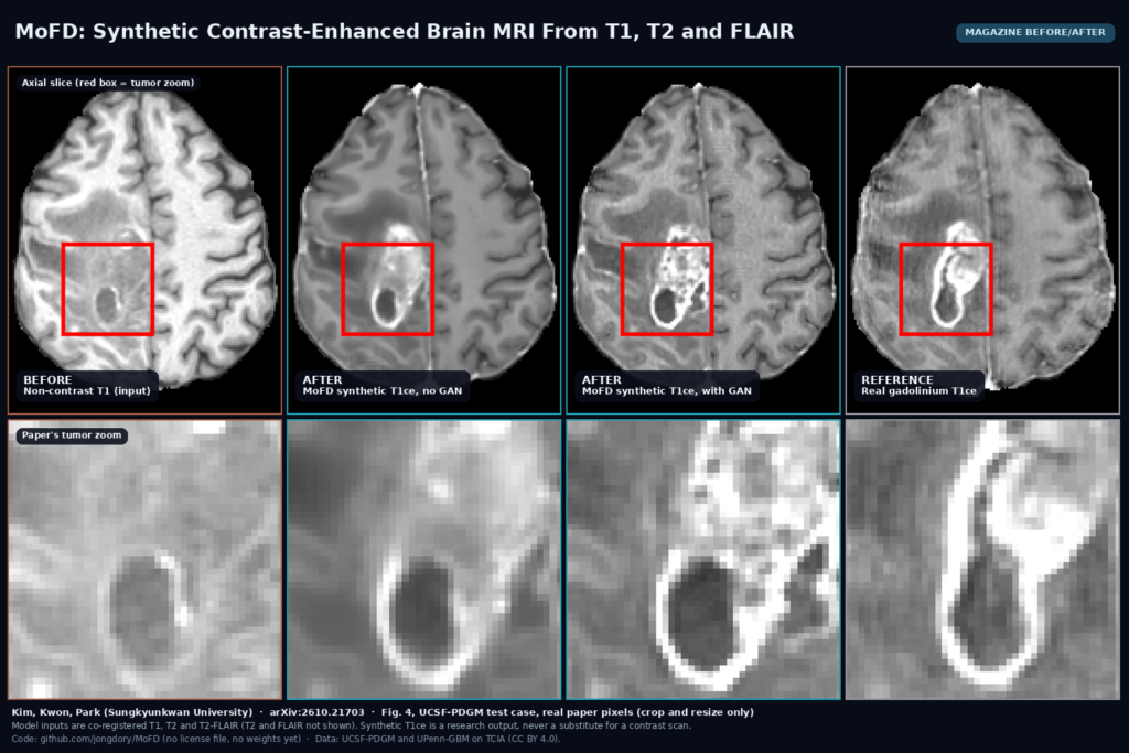
Brain tumour MRI protocols usually include a gadolinium injection and a post-contrast T1 scan, because on that scan the enhancing tumour and its boundaries stand out from edema and normal tissue. The pre-contrast T1, T2 and FLAIR images are already on the scanner before the injection. Jonghun Kim, Junmo Kwon and Hyunjin Park of the Department of Electrical and Computer Engineering at Sungkyunkwan University in Suwon, Korea, posted arXiv:2610.21703 on 15 October 2026 (accepted at ACCV 2026). Their model, MoFD, takes those three non-contrast sequences and predicts the contrast-enhanced T1 (T1ce) volume. The code is public at jongdory/MoFD, and both training datasets are public on The Cancer Imaging Archive under CC BY 4.0.
Why a viewer team should care
The paper’s motivation is clinical. Gadolinium may not be fully excreted and can accumulate in brain and bone, and a contrast scan adds acquisition time and cost. For a team that builds viewers and analysis pipelines, the more immediate use is a missing-sequence problem. BraTS-style brain tumour segmentation models expect four sequences, T1ce included, and real archives often lack one. A synthetic T1ce, clearly labelled as such, can fill that slot for research, retrospective studies and triage experiments. It is something you hang next to the real sequences with a loud label, and it should never be read as a contrast study.
What goes in and what comes out
Input is a co-registered set of T1, T2 and T2-FLAIR volumes from one brain MRI study. The authors’ data were skull-stripped, registered to the same anatomical template and resampled to 1 x 1 x 1 mm voxels before training. The paper reports cropping to 192 x 192 x 128; the released data loader crops to the T1 foreground and then pads or center-crops to 192 x 192 x 96, and rescales each sequence from its 0th to 99.5th intensity percentile into the range -1 to 1. Output is one synthetic T1ce volume on that cropped grid, written as NIfTI by sampling.py. The model is fully 3D and processes the whole cropped volume in one pass.
How it works
Most earlier models stack the source sequences as input channels and let one encoder sort them out. MoFD runs each sequence through its own pass of a shared-weight 3D U-Net encoder (feature widths 32, 64, 128, 256 and 512), so T1, T2 and FLAIR land in the same feature space but stay separate. At every skip connection the MoFD module then builds six feature maps for that scale: the three sequence features and the three pairwise differences (T1 minus T2, T1 minus FLAIR, T2 minus FLAIR). The differences are there because the sequences disagree in informative ways. Fluid, edema and lesion change brightness differently on T1, T2 and FLAIR, and the authors argue that raw channel stacking is sensitive to intensity scaling and noise, while differences computed in feature space describe how contrast changes between sequences.
Each of the six maps goes through a normalized convolution block, then global average pooling and a softmax turn them into weights, and the decoder receives their weighted sum. Training uses an L1 loss against the real T1ce plus a structural alignment loss, the structure term of SSIM computed between the features of different sequences, which pushes the encoder to agree on anatomy across contrasts. An optional PatchGAN discriminator adds an adversarial loss. The paper reports results with and without it.
What the numbers say
The training splits held 210 subjects from each of UCSF-PDGM and UPenn-GBM, and the authors compared MoFD against seven published synthesis models, including ResViT, Hi-Net and a 3D latent diffusion model (ALDM). On the 54 UCSF-PDGM test subjects, the regression variant without the GAN scored the highest PSNR (25.00 dB, against 24.54 dB for the best baseline, from Chen et al.) and the highest SSIM (Table 1). The GAN variant had the best perceptual score but lower fidelity. The authors also tested the images downstream. They trained an nnU-Net on real T1ce images and ran it on the synthetic ones. On the regression variant’s output it reached an average Dice of 0.741 across whole tumour, enhancing tumour and tumour core, the best of all methods, while the same network scored 0.811 on the real T1ce (Tables 1 and 3). The gap sits mostly in the tumour core, 0.588 against 0.840. In the loss ablation, the regression model segmented better than the GAN model, and the authors read that as the adversarial loss adding realistic detail that is not in the patient.
The figure
The featured image uses the top row of Fig. 4, one UCSF-PDGM test case. From left to right are the non-contrast T1 input, the MoFD output without and with the GAN loss, and the real gadolinium T1ce. The bottom row repeats the paper’s zoom on the tumour. On the pre-contrast T1 the lesion is a dark cavity with a faint rim. Both MoFD outputs draw a bright enhancing rim around it. The regression output is smooth and keeps the rim shape. The GAN output is sharper but fills the area above the cavity with bright speckled texture that the real scan does not have there. The real T1ce shows an enhancing rim that extends upward beyond the cavity, and neither synthetic image reproduces that extension cleanly.
Limits
The paper evaluates on two public glioma collections only, with no external hospital, no other pathology and no reader study. Every input was co-registered to a template and skull-stripped before the model saw it, so a raw clinical study needs that full preprocessing chain first. The tumour core result shows where a synthetic contrast image is weakest. The network has to infer enhancement from how the other sequences look, so a small or atypical enhancing focus can be missed or invented. In the paper’s own Fig. 4, three of the baseline methods lose the tumour core almost entirely on that case, and MoFD’s synthetic core is still well short of the real one in Dice.
The released code has its own gaps. There are no trained weights yet; the config leaves the checkpoint path to be filled. The split CSV files the loader reads are not in the repository. The dataset loader skips any subject that has no real T1ce file, so running it on a case that never had contrast needs a small code change. The shipped config trains with the adversarial term on from the first step; for the regression variant you would turn the discriminator factor off in the loss settings yourself. sampling.py writes the output NIfTI with the source orientation and spacing but on the cropped grid with a zero origin, so it will not overlay on the original series until you undo the crop.
Code, data and license
The repository holds the training script, a sampling script, the MoFD module and a config for the brain task. It builds on the nnU-Net team’s architecture package (dynamic_network_architectures, imported but not listed in requirements.txt) and MONAI 1.2 (pinned in environment.yaml). There is no license file, which by default means the authors keep all rights. Treat it as code you can read and test, and ask the authors before you put it in a product. UCSF-PDGM and UPenn-GBM are both distributed by TCIA under CC BY 4.0, which permits commercial use with attribution and TCIA’s data use policy, so retraining on them is possible once the code license is clear.
How we would wire it into a viewer
We would run it as a research job outside the viewer. When a brain tumour study arrives with T1, T2 and FLAIR but no post-contrast T1, convert the series to NIfTI, run skull stripping and co-registration as the authors did, and run MoFD on a GPU worker. Then undo the crop, resample back to the T1 grid, and write the result as a new derived series with ImageType DERIVED\SECONDARY, a series description such as “Synthetic T1ce (AI, MoFD, not a contrast scan)” and a reference to the source series. In the viewer, show it only in a research or segmentation workflow, with a banner on the viewport, and keep it out of the default hanging protocol for diagnostic reads. If the main consumer is a downstream segmentation model, check that model’s Dice on synthetic inputs against real T1ce on your own cases first, because the tumour core gap in the paper is large. For background, see what a DICOM viewer does, our guides on DICOM to NIfTI and NIfTI back to DICOM, and our earlier post on tumour overlay confidence when MRI sequences are missing.
Sources
- Kim, J., Kwon, J., Park, H. Mixture of Multi-Sequence Feature Difference for Contrast-Enhanced MRI Synthesis. arXiv:2610.21703, 2026 (ACCV 2026). https://arxiv.org/abs/2610.21703. PDF: https://arxiv.org/pdf/2610.21703.
- Code (no license file at the time of writing): https://github.com/jongdory/MoFD.
- Datasets (CC BY 4.0): UCSF-PDGM, https://www.cancerimagingarchive.net/collection/ucsf-pdgm/. UPenn-GBM, https://www.cancerimagingarchive.net/collection/upenn-gbm/.
- Featured image: Fig. 4 of arXiv:2610.21703, real paper pixels, cropped and resized only.