
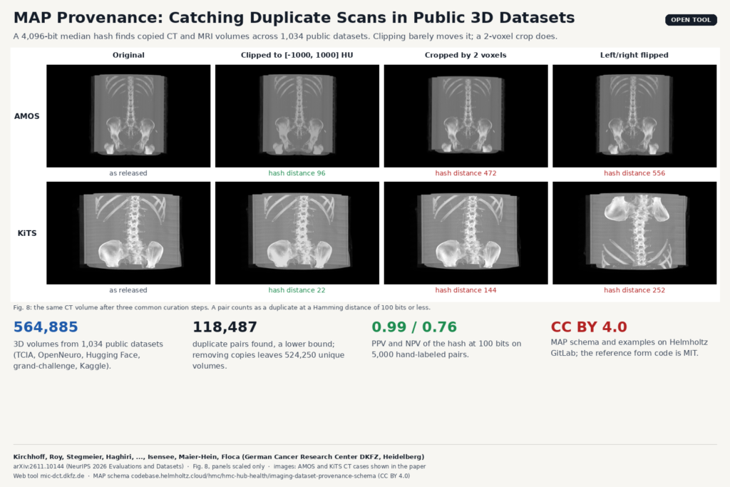
Most segmentation models you can download today were pretrained or benchmarked on some mix of public CT and MRI datasets. That mix is rarely as independent as it looks. A paper from the Division of Medical Image Computing at the German Cancer Research Center (DKFZ), arXiv:2611.10144, accepted at the NeurIPS 2026 Evaluations and Datasets track, measures how much the public 3D imaging ecosystem reuses itself. The authors, led by Yannick Kirchhoff, Saikat Roy, Elisa Stegmeier and Hamideh Haghiri with Fabian Isensee, Klaus Maier-Hein and Ralf Floca among the senior authors, gathered 1,034 public datasets, hashed every volume, and traced the copies. They also release a small JSON profile called MAP (Metadata for Aggregation and Provenance) so that dataset builders can write down where their data came from.
What the paper does
The authors call large aggregations of public datasets “dataset collections” and separate them from curated multi-center cohorts such as PI-CAI. A collection like AbdomenAtlas, CADS, FLARE or OpenMind exists to scale training, so it pulls in whatever public data fits, and those sources often already contain each other. Their first example is AbdomenCT-1K, which aggregates KiTS19, LiTS (also released as MSD Task 03), MSD Pancreas, MSD Spleen and NIH Pancreas. LiTS also sits inside CT-ORG, and both CT-ORG and AbdomenCT-1K were later folded into AbdomenAtlas 1.1. In a second example, FLARE23 and DAP-Atlas both include AutoPET, so training on one and testing on the other quietly breaks independence.
To measure this at scale they built their own collection of 564,885 3D volumes from TCIA, OpenNeuro, Hugging Face, grand-challenge and Kaggle. The 782 OpenNeuro datasets are treated as one, which leaves 253 datasets for the analysis.
How the duplicate search works
The authors kept the hash simple on purpose. Each volume is resampled to a 16 × 16 × 16 grid, every voxel is set to 1 if it is above the volume’s median intensity and 0 otherwise, and the result is flattened into a 4,096-bit code. Two codes are compared by Hamming distance, and an Annoy approximate nearest-neighbor index (1,024 trees) avoids comparing every pair. A pair counts as a duplicate at a distance of 100 bits or less.
Because the median threshold ignores absolute intensities, the hash survives HU clipping, which is the most common change a curator makes. It needs no DICOM headers or patient identifiers, and the 4,096-bit code can be shared without sharing the image. The authors checked the approximate search against an exhaustive one on 50,000 random volumes: for 99.8% of the images that had a cross-dataset match within 100 bits, the index found the closest one.
What they found
The final count is 118,487 duplicate pairs. Hashing found 56,051 of them (44,727 with identical hashes), and the other 62,436 came from dataset-specific variants of the search, such as clipping before hashing, and from manual tracing of known overlaps. In total 64,888 volumes have at least one copy elsewhere. Removing the extra copies takes the collection from 564,885 to 524,250 unique volumes, a 7.2% drop. At least partial overlap shows up for 136 of the 253 datasets, and the largest connected group in the overlap graph links 107 datasets, including AMOS, KiTS, LiTS, AbdomenCT-1K, FLARE and AbdomenAtlas.
The authors are clear that 118,487 is a lower bound. They hand-labeled 5,000 candidate pairs: of the 1,000 pairs the pipeline flagged, 989 were real duplicates (positive predictive value 0.99), but of the 4,000 it did not flag, 974 were also duplicates (negative predictive value 0.76). Most of the misses were cropped or clipped copies, different contrast phases of one study, or CT reconstructed with a different kernel. The authors counted those last two as duplicates because they carry the same leakage risk.
Why a medical imaging team should care
If you fine-tune on one public collection and report results on another, a share of your test cases may already be in your training set. The paper adds that cross-validation inside a collection has the same problem, since folds can share copies of the same scan. Scaling curves also look better than they should when part of the extra data is repeated data.
For a team that builds viewers and segmentation tools on public data, the practical uses are:
- Before training. List every public source behind your pretraining data and your evaluation data, and look up their known overlaps on the project site before you trust a held-out number.
- When a client hands over data. Hospitals sometimes contribute to public challenges. A local hash of their export, checked against the public reference, tells you whether some of their “private” test cases are already public. The hashing runs on your machine and only the 4,096-bit codes would be uploaded.
- When you release data. Fill in a MAP profile and ship the JSON with the release, so the next team can see which sources you reused, which parts, what you changed and how you handled duplicates.
- Inside your own pipeline. The paper recommends keeping DICOM SOP Instance UIDs as auxiliary metadata whenever you convert to NIfTI. They are the only identifier that matches exact copies reliably, and they are lost in most public releases.
Where it falls short
- Spatial changes break the hash. In a controlled test on 883 CT scans, clipping to [−1000, 1000] HU kept 96.2% of copies within the threshold, but cropping or padding by only 2 voxels per side dropped that below 9%. Left and right flips also push the distance far past 100 bits in two of the three examples in the paper.
- The hash depends on how you load the image. Orientation handling, resampling and format conversion change the code, so your local loader has to match the reference pipeline.
- Similarity is not lineage. A match says two volumes look alike. It does not say which dataset copied which, or what happened to the labels.
- MAP is self-reported. It records what curators know and does not detect anything by itself. It also works at dataset and collection level, not per case.
- The duplicate check is not open yet. On 10 November 2026 the site’s hash index reported 526,134 hashes from 972 datasets, but the upload check and the hash script download were marked “coming soon”. The dataset explorer with its overlap table and the MAP form were already usable.
Links and license
The web tool is at mic-dct.dkfz.de, with the MAP form at mic-dct.dkfz.de/metadata. The MAP schema, controlled vocabularies (mapped to RadLex and DICOM codes) and example profiles are on the Helmholtz GitLab at hmc/hmc-hub-health/imaging-dataset-provenance-schema, under CC BY 4.0, while the reference form app is MIT. The paper itself is CC BY 4.0. No images are hosted on the site, and each source dataset keeps its own license, so check each source’s terms before you reuse anything listed in the overlap table.
Paper: arXiv:2611.10144 · Web tool: MIC-DCT · MAP schema: Helmholtz GitLab (CC BY 4.0, form code MIT)