
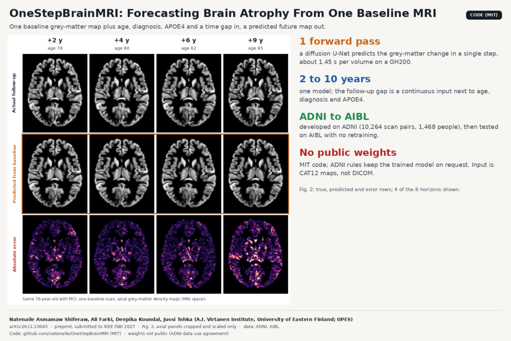
Memory clinics already measure atrophy. They take a T1-weighted MRI, run it through a segmentation or morphometry tool, and compare regional volumes against norms or against the patient’s last scan. What they cannot do is look forward: show a patient, or a trial sponsor, where grey matter is likely to be lost over the next few years. A group at the University of Eastern Finland built a model that tries to do that from a single baseline scan. It is described in arXiv:2611.10043, and the code is public under the MIT license. The paper does not give the model a name; the repository calls it OneStepBrainMRI, so we use that here.
What OneStepBrainMRI does
The input is one grey-matter density map computed from a baseline T1 scan, plus four facts about the person: age, diagnosis (cognitively normal, mild cognitive impairment or dementia), the number of APOE4 alleles (0, 1 or 2), and how many years ahead you want to look. The output is a predicted grey-matter density map for that future date, in the same space as the input.
The maps come from CAT12, the Computational Anatomy Toolbox, version 12.8.1. They are modulated maps normalized to MNI space at 1.5 mm isotropic resolution, 113 × 137 × 113 voxels. Because they are modulated, summing a region gives that region’s grey-matter volume, so a predicted map can be turned back into predicted regional volumes.
One model covers every horizon from 2 to 10 years. The time gap is a continuous number fed to the network, so you do not train one model per horizon.
How it works
First, the network predicts the change between visits. The target during training is the follow-up map minus the baseline map, and at inference the predicted change is added back to the baseline. Most anatomy carries over from one visit to the next, so the network spends its effort on the difference. In the ablation, predicting the whole follow-up image directly gave the weakest result of all variants.
Second, it is a diffusion model that runs a single step. Training follows a standard denoising diffusion setup with 1,000 noise levels, using a 3D version of the ADM U-Net from OpenAI’s guided-diffusion (about 716M parameters). The network is trained to output the clean change map directly at any noise level. At inference it gets pure noise, the baseline map and the covariates, and its first and only output is taken as the answer. There is no iterative sampling. The README reports 1.45 seconds per volume on one NVIDIA GH200, and 1.80 seconds including NIfTI read and write, measured over 1,568 test pairs. Repeated runs on the same hardware give bit-identical output.
Third, the loss rewards getting the spatial pattern right. Voxel-wise mean squared error is combined with a Pearson correlation term between predicted and true change, both computed inside the grey-matter mask. The authors’ point is that squared error alone does not capture where the change happens. Removing the correlation term lowered the main score from 0.478 to 0.456.
The covariates (age, diagnosis, APOE4 count, time gap) go through a small MLP and are added to the diffusion timestep embedding. Dropping them lowered the score to 0.461.
What they tested it on
Development data came from ADNI: 10,264 baseline and follow-up scan pairs from 1,468 people, with gaps from 2 to 10 years, split by participant into 1,028 for training, 220 for validation and 220 for testing. External testing used AIBL, 332 pairs from 150 people at 3 and 6 years, with no retraining. The ADNI cohort was 40% cognitively normal, 49% MCI and 11% dementia; AIBL was 79%, 15% and 6%.
The main metric is Δ-Pearson: the spatial correlation, within grey matter, between the change the model predicted and the change measured at follow-up. On the ADNI test set it was 0.478 overall, and 0.450 on AIBL. Regional Δ-Pearson was 0.503 in the hippocampus and 0.509 in the entorhinal cortex, two regions the authors single out as relevant to neurodegeneration. Correlation went up with the horizon, from 0.444 at 2 years to 0.582 at 10 years, while voxel-wise errors also grew. The authors read this as the pattern of change becoming clearer over long gaps even as its exact size gets harder to hit.
The featured image shows Fig. 2 of the paper: one ADNI test participant, 76 years old with MCI and no APOE4 allele, predicted from a single baseline scan. The top row is the follow-up map that was measured, the middle row the prediction, and the bottom row the absolute error. The error map gets brighter toward 9 years, matching the larger errors at long horizons in the paper’s table.
Why a viewer or clinic team should care
Most neuro products in a PACS or a research viewer stop at the present tense: volumes, percentiles, maybe a comparison with the prior study. A forecast map fits next to those as one more overlay. For a given patient you could show the baseline map, the predicted map at 3 or 5 years, and the predicted change as a heat map on the T1, with the hippocampus and entorhinal cortex summarized as numbers. At under two seconds per volume, it runs fast enough to sit inside an existing post-processing job.
Research groups and trial teams are the likelier first users. A model that predicts each person’s expected change could be used to pick participants who are likely to decline within a trial’s window, or as a reference trajectory to compare an observed follow-up against. Neither use is tested in this paper.
The engineering cost sits in the preprocessing. The model does not read DICOM. You would export the T1 series to NIfTI, run CAT12 with the same version and settings, and check that the output is 113 × 137 × 113 at 1.5 mm with values up to about 1.2. Then the prediction has to be warped back from MNI space to the patient’s native scan if you want to overlay it on their images. The repository is explicit that two constants (a change scale of 0.22 and the ADNI age mean and standard deviation) must not be re-estimated on new data if you use weights trained on ADNI.
What it does not tell you yet
- Weights are not public. Under the ADNI data use agreement, the authors share them on request with researchers who have their own ADNI access. Anyone else retrains from scratch, which took about 50 hours on two GH200 GPUs.
- The output is a grey-matter density map. It forecasts tissue loss and says nothing about diagnosis or cognition.
- A Δ-Pearson around 0.48 means the spatial pattern is partly right. Do not read a single patient’s forecast as a prognosis.
- Training data is unevenly spread. Most pairs are at 2 to 4 years, and only 149 ADNI pairs reach 10 years. The authors flag that under-represented intervals and diagnostic groups are hard to evaluate.
- Both cohorts are research studies of older adults (mean baseline age about 73 in ADNI). Routine clinical scans and younger patients are untested.
- It is a short conference submission to IEEE ISBI 2027 and has not been peer reviewed yet. The results compare the model with its own ablations only, with no other forecasting method as a baseline.
How to try it
The repository at github.com/natenaile/OneStepBrainMRI has training, inference and evaluation scripts with YAML configs, the ablation configs from the paper, and a DATA.md file that spells out the expected inputs: CAT12 modulated grey-matter maps, a CSV of scan pairs with diagnosis, APOE4 count and normalized age, and the two normalization constants. It was tested with Python 3.12 and PyTorch 2.10. The evaluation script reports global and regional metrics per interval using the Neuromorphometrics atlas.
Intervals outside the 2 to 10 year training range are accepted, but the authors ask that those be reported separately as extrapolation. The code is MIT and covers the source only, not the ADNI or AIBL data or weights trained on them. For other forecasting work on the blog, see the post on forecasting CSF tracer maps from pre-contrast brain MRI, and for the viewer side, building a custom neuroimaging DICOM viewer.
Source and license
Paper: Natenaile Asmamaw Shiferaw, Ali Farki, Deepika Koundal and Jussi Tohka, “Covariate-Conditioned One-Step Diffusion for Multi-Horizon 3D Brain MRI Prediction in Aging and Neurodegeneration”, arXiv:2611.10043 (eess.IV, 5 November 2026), submitted to IEEE ISBI 2027. All authors are with the A.I. Virtanen Institute for Molecular Sciences, University of Eastern Finland, Kuopio; Deepika Koundal is also with the University of Petroleum and Energy Studies (UPES), Dehradun, India. Code: github.com/natenaile/OneStepBrainMRI, MIT, built on OpenAI’s guided-diffusion. Weights: not public; available on request to researchers with ADNI access. Data: ADNI and AIBL under their own data use agreements. Featured image: Fig. 2 of the paper, axial panels for 4 of the 8 horizons, cropped and scaled.