
MR elastography is one of the few MRI techniques that measures a mechanical property instead of a signal. A pneumatic actuator under the patient’s head vibrates at a few tens of hertz, shear waves travel through the brain, motion-encoding gradients write the tiny displacements into the phase of the MR signal, and an inversion algorithm turns the wave pattern into a shear wave speed map. Stiffer tissue carries faster waves. It is also slow. Every slice needs several vibration phases, several encoding directions and often several frequencies for every slice, and the inversion is itself sensitive to noise. Stefan Martin, Andreas Kofler and colleagues at Physikalisch-Technische Bundesanstalt (PTB) and Charité Berlin (arXiv:2611.26111, posted 19 November 2026, accepted in IEEE Transactions on Biomedical Engineering) speed this up by training the reconstruction network against the stiffness map itself.
The network reconstructs heavily undersampled spiral data, then a standard inversion called k-MDEV computes the shear wave speed, and during training the error on that final map flows back into the reconstruction. The repository is named E2E-MRE, which is the label we use here.
Why image quality is the wrong target here
In most accelerated MRI work, success means the reconstructed image looks like the fully sampled one. In MRE, the image is only an intermediate product. What matters is the phase, because that is where the wave lives, and the inversion takes spatial derivatives of that phase. Small phase errors that a reader would never notice on a magnitude image get amplified into speckle in the stiffness map. A reconstruction tuned for pretty magnitude images can still produce a poor elastogram. The paper’s total variation baseline is an example. TV visibly cleans up magnitude images, yet its stiffness maps are only slightly better than those from iterative SENSE.
How the pipeline works
Acquisition. The target protocol uses a single-shot spiral readout, so each vibration phase and encoding direction can be captured in one shot. Spiral arms are rotated by the golden angle across time points, directions and frequencies, so each time frame samples a different part of k-space. The model handles one, two or three spiral arms of 863 points each, which the authors equate to undersampling factors of about 19, 9.5 and 6.3.
Reconstruction. The network is an unrolled scheme in the MoDL style. It starts from an approximate pseudo-inverse of the multi-coil spiral data, then alternates six times between a CNN that removes artifacts and a data-consistency step solved with conjugate gradients, so the output never drifts far from the measured k-space. The CNN is XTYT, a 2D U-Net applied to x-t and y-t slices of the image series, which exploits the fact that a propagating wave is highly correlated across the eight vibration phases. The six-iteration version has about 2.1 million parameters. Operators come from MRpro, the group’s open PyTorch MR reconstruction package.
Inversion as a layer. k-MDEV (Tzschätzsch and colleagues, 2016) extracts the phase, unwraps it, takes a temporal Fourier transform to isolate the vibration frequency, applies directional filters to separate waves travelling in different directions, and estimates the wave number from phase gradients. It has no learnable parameters, but the authors implemented it as a differentiable module so gradients can pass through it.
Two-stage training. The network is first pre-trained for 50 epochs on images alone. It is then fine-tuned for another 50 epochs with a combined loss weighted 0.1 on images and 0.9 on the stiffness map, computed inside a brain mask so the network does not spend its effort removing artifacts outside the head. Keeping a small image term stops the network from forgetting how to produce readable magnitude and phase images. Dropping that weight from 0.15 to zero improved the stiffness metrics slightly and made image reconstruction 12% worse.
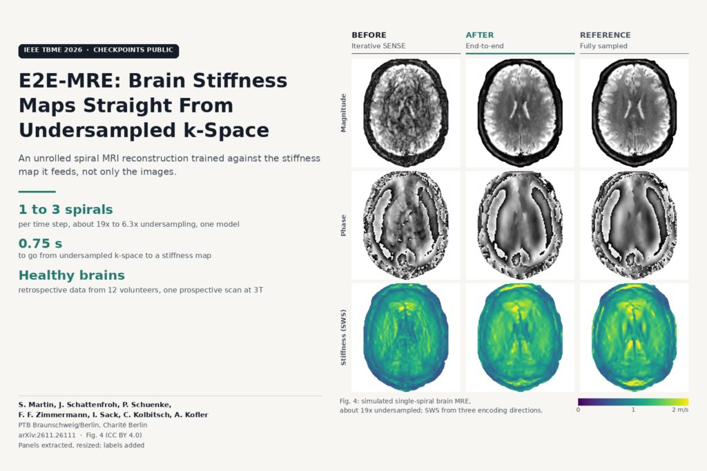
The featured image above is Fig. 4 of the paper: magnitude, phase and stiffness for one simulated single-spiral slice, comparing iterative SENSE, the end-to-end model and the fully sampled reference.
What the results show
The data came from 13 healthy volunteers scanned at Charité on a 3T Siemens Magnetom Lumina with a 32-channel head coil and a pneumatic actuator under the head, driven at 20, 25, 30 and 35 Hz. Twelve volunteers had a fully sampled Cartesian brain MRE scan (40 slices at 1.6 x 1.6 x 2 mm, 451 seconds per subject), and spiral acquisitions were simulated from it, with coil maps deliberately estimated from a small calibration region to mimic real-world mismatch. Training, validation and test used 8, 1 and 3 subjects.
At a single spiral arm, the hardest setting, the stiffness maps from the end-to-end model reached SSIM 0.93 and NRMSE 0.14 against the fully sampled maps, compared with 0.87 and 0.20 for TV and 0.83 and 0.23 for iterative SENSE. That NRMSE gap to TV is the 30% reduction the abstract quotes. With two or three spiral arms all methods improve, and the ranking stays the same.
The end-to-end fine-tuning itself buys about 5% lower stiffness-map error over the image-only pre-trained network. That is a modest gain, and the authors say so: most of the improvement over classical methods comes from having a learned, data-consistent reconstruction at all. Six unrolled iterations beat a single large iteration by 18% on stiffness quality.
The thirteenth volunteer was scanned prospectively with a new spiral MRE sequence written in PyPulseq, single 5 mm slice, with 25 spiral arms acquired as the reference. Using only one to three arms, the model produced maps that resemble the 25-arm reference. With one arm they lack fine detail; with two or three they match it closely. Once trained, going from undersampled k-space with eight vibration phases to a stiffness map takes about 0.75 seconds.
Where it falls short
- Healthy brains only. All 13 subjects were healthy volunteers. The authors argue that data consistency and an established inversion make failure on pathology unlikely, but there is no tumour, hydrocephalus or neurodegeneration case in the paper.
- Mostly simulated undersampling. The quantitative tables come from spiral data simulated from Cartesian scans of 12 subjects, with 3 in the test set. The in vivo check is one volunteer, one slice, judged visually.
- The reference is not ground truth. The 25-arm in vivo reference may carry spiral errors from gradient imperfections, which the authors leave to future work.
- 2D and brain only. Reconstruction is per slice over time. Extending it to 3D or to the liver, where breathing makes speed most valuable, is listed as future work.
- Training cost. Pre-training took about 3 days and fine-tuning about 4 days on one NVIDIA A6000, with 35.4 GB of GPU memory during fine-tuning. That is fine for a research group, less so for a site retraining for its own scanner.
- Inversion assumptions carry over. k-MDEV assumes locally planar waves and local homogeneity, and those assumptions hold least well where stiffness changes abruptly. The network does not change that step.
Where it fits for an MRI platform
For a team building MRI reconstruction or viewer software, the paper is a clean example of training a reconstruction for the number the clinician will read. Elastography makes a good test case because the final map sits so many processing steps away from the raw image. The same structure applies to T1 mapping (the group’s earlier PINQI work) or any quantitative map computed from a series of images: make the parameter fitting differentiable, put it after the reconstruction, and fine-tune on the map.
The authors see sub-second stiffness maps from single-shot spirals as a route to free-breathing abdominal MRE, faster pediatric scans and dynamic studies of brain stiffness. In a viewer, the output is a familiar shear wave speed overlay in m/s that can sit next to the magnitude series. Any deployment would need its own sequence, its own calibration and patient validation first.
Code, weights and licence
The paper links Stef-Martin/E2E-MRE. When we checked on 22 November 2026, the repository contained the training and testing scripts, network modules, patched MRpro operators and two checkpoints (a six-iteration model of about 25 MB and a single-iteration model of about 99 MB, whose file names indicate the 0.1 image weight). There is no licence file, so reuse rights are unclear. The README says the training data are not yet on Zenodo, that the scripts are not runnable until they are, and that the shear wave speed calculation code is intentionally excluded and will not be released on GitHub. You can inspect the reconstruction network today, but reproducing the stiffness maps needs your own k-MDEV implementation. The paper itself is released under CC BY 4.0.
Source
Stefan Martin, Jakob Schattenfroh, Patrick Schuenke, Felix Frederik Zimmermann, Ingolf Sack, Christoph Kolbitsch and Andreas Kofler, “Physics-Informed Deep Learning for Shear Wave Speed Estimation in MR Elastography”, arXiv:2611.26111 (v1 19 November 2026), authors’ accepted version of the IEEE Transactions on Biomedical Engineering article (DOI 10.1109/TBME.2026.3666306). Affiliations: Physikalisch-Technische Bundesanstalt (PTB), Braunschweig and Berlin, and Charité Universitätsmedizin Berlin. Featured image: Fig. 4 of the paper (magnitude, phase and shear wave speed for iterative SENSE, the proposed method and the fully sampled reference), panels extracted from the PDF, resized, with labels added.