
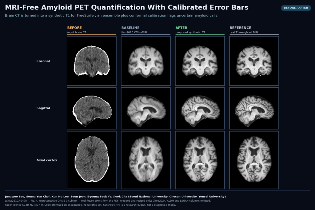
Amyloid PET quantification usually needs a T1-weighted MRI. FreeSurfer parcellates the MRI, the regions are mapped onto the PET, and the standardized uptake value ratio (SUVR) is computed against the cerebellar cortex. Some patients reach the PET scanner without a usable MRI, because of a contraindication, claustrophobia, motion or the burden of one more exam. A PET/CT exam already includes a low-dose CT of the head. In arXiv:2610.40478, Jungwoo Seo, Seung Yun Choi, Kun Ho Lee, Seun Jeon, Byoung Seok Ye and Jiook Cha (Seoul National University, Chosun University in Gwangju and Yonsei University) turn that CT into a synthetic T1, run the normal MRI pipeline on it, and attach a calibrated interval to every SUVR that shows when the number can be trusted.
What the method does
The synthesis model is a Brownian Bridge diffusion model built on the slice-consistent version from Choo et al. (2024). The authors made three changes to it, all aimed at the fact that grey and white matter barely separate on CT.
- More training data. They trained one model on 1,130 CT and MRI pairs pooled from OASIS-3, the brain subset of SynthRAD2023 and an in-house cohort from Severance Hospital in Seoul.
- A data-source label. They feed the model the name of the source dataset at every denoising step, so scanner and protocol differences between the three sources do not blur the mapping.
- Wider CT context. The model reads 15 consecutive axial CT slices to predict the central three T1 slices. In their ablation this through-plane context gave the largest gain.
At inference the model has no access to the patient’s MRI. Its style condition is the mean MRI intensity histogram of the training subjects, and the full 3D volume is assembled with the slice-consistent sampling of Choo et al. They also tried a frozen segmentation teacher as extra supervision and dropped it because it added nothing significant.
The workflow on one patient
- Clip the PET/CT head CT to [-100, 200] HU and align it rigidly to MNI152 space, with a brain mask taken from the CT.
- Generate a synthetic T1 with each of five independently trained copies of the model.
- Run FreeSurfer recon-all (7.2.0 in the paper) on each synthetic T1, register the PET to it, and compute regional SUVRs with the cerebellar cortex as reference. The headline number is the mean cortical SUVR (MCSUVR) over precuneus, prefrontal cortex, gyrus rectus and lateral temporal cortex.
- Take the mean of the five SUVRs as the estimate and their standard deviation as the uncertainty scale.
- Widen that spread by a factor learned with split conformal prediction on a calibration set (93 OASIS-3 subjects with same-day PiB PET and MRI). The result is an interval that should contain the SUVR you would have got from the real MRI at the chosen coverage, here 90%.
- Compare the interval with the amyloid cut-off of MCSUVR 1.42 for PiB. Entirely below reads as confidently negative, entirely above as confidently positive, and an interval that straddles 1.42 is marked indeterminate.
What a viewer would hang on the scan
A reading tool built on this would show the PET over a synthetic T1 with FreeSurfer regions, a table of regional SUVRs, and the MCSUVR with its interval and one of three labels: negative, positive or needs MRI. The synthetic T1 should carry a visible “synthetic, not for diagnosis” banner. It exists to place regions on the PET, and nobody should read it as a brain MRI.
Results that matter for a clinic
On the 87 OASIS-3 test subjects with PiB PET, the MCSUVR from a single synthetic MRI (one model, no ensemble averaging) differed from the real-MRI value by a mean absolute error of 0.016 (SD 0.015), with a Pearson r of 0.9987. Every one of the 87 got the same amyloid-positive or negative call as with the real MRI. For comparison, a PET-only template pipeline built from OASIS-3 had an MAE of 0.131 and 96.6% concordance, and the strongest earlier CT-to-MRI model (Choo2024) reached 0.021.
At 90% target coverage, 80 of 87 real-MRI values fell inside their interval (92.0%), and 85 of 87 subjects got a confident call. The two indeterminate patients had ensemble means of 1.4103 and 1.4473, both close to the cut-off. When the authors moved the cut-off between 1.30 and 1.50, every disagreement with the real-MRI call landed in the indeterminate group.
Where it breaks
- Calibration does not travel. On the external GARD cohort (84 subjects, 18F-florbetaben, GE Discovery ST and STE PET/CT), the synthesis model held up zero-shot, but the OASIS-3 intervals covered only 62.2% of real-MRI values at the 90% target. Recalibrating on GARD subjects brought coverage back to 90.7% (SD 6.2% over 1,000 random splits) and widened the mean MCSUVR interval from 0.119 to 0.203. Each split used paired CT, MRI and PET from 41 subjects, so a new site needs its own small calibration set.
- Medial cortex is harder. Regional errors are larger in the precuneus and the anterior and posterior cingulate, where folding is complex and CT shows little. The anterior cingulate interval averaged 0.185 SUVR units wide, against 0.069 for parietal cortex.
- The source label is a workaround. GARD had no label of its own, so the team used the OASIS-3 label because its CT looked closest. That choice will not generalise to every new scanner.
- Abnormal brains are untested. The training data does not systematically include tumours or large white-matter lesions, and the authors warn that a synthesis model can erase pathology it has rarely seen. A wrong synthetic anatomy moves the regions and therefore the SUVR.
- Selected, retrospective cohorts. The PET analysis kept only same-day PET and MRI pairs that passed quality control, there was no analysis by age, sex or ethnicity, and external validation covers one cohort and two tracers in total.
- Compute. Five synthetic MRIs per patient means five diffusion runs and five FreeSurfer recon-all runs before you have one SUVR with an interval.
Code, weights and licence
The paper says code will be released on acceptance at github.com/Transconnectome/CT-to-MRI-PETQ-UQ. That repository was not public when I checked on 30 October 2026, and I found no released weights. OASIS-3 is available under its data use agreement and SynthRAD2023 under CC BY-NC 4.0. The Severance and GARD cohorts are not public. The preprint is licensed CC BY-NC-ND 4.0 and was submitted to Medical Image Analysis. This is a research result and not a cleared clinical tool.
My take
The accuracy is good, and the decision rule is what I would copy. Five models you already trained, plus one conformal factor fitted on 93 calibration subjects, give each SUVR a range and tell the reader which patients still need an MRI. The GARD result shows the catch: that factor belongs to the cohort it was fitted on. Before using this at a new site I would collect a local calibration set with real MRI, check coverage on it, and keep the interval visible next to the number in the viewer.