
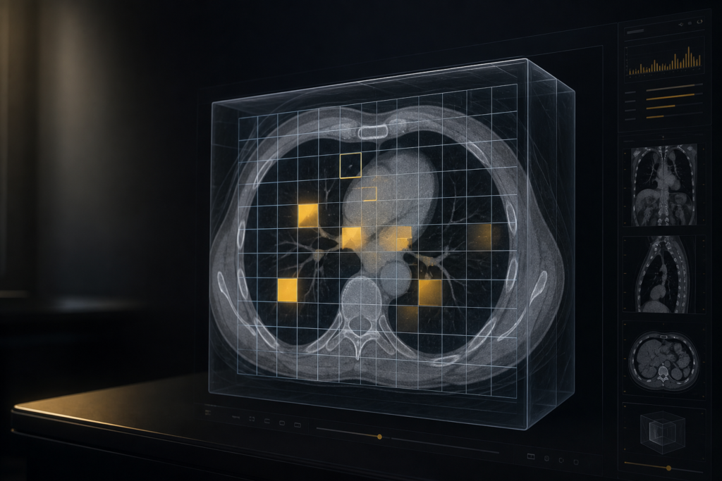
Chest CT AI is no longer short on image-level labels. CT-RATE already gives you tens of thousands of non-contrast studies with report-derived findings. What most product teams still cannot do well is the next step: put the finding on the volume.
That is the gap PatchChestCT is built for. Published in Scientific Data on 12 August 2026, it adds physician-reviewed 3D patch-level labels for nine abnormalities across 2,201 CT-RATE studies, one reconstructed volume per study. The labels are meant as spatial supervision you can train against, not as another “present / absent” leaderboard.
If you ship DICOM viewers or segmentation platforms, that distinction is operational. A model that only says “consolidation” is a badge. Once it lights a region in the viewport, it is a tool.
Image-level findings are not localization
Most public chest CT resources still stop at the study. The report mentions atelectasis, an NLP pipeline flips a label, and the training objective becomes multi-label classification. That is useful for triage and retrieval. It is a weak signal for anything you would overlay in a viewer.
Weak supervision can extract a heatmap. The PatchChestCT baselines show how far that usually gets you. Across 3D ResNet-18, Swin3D-T, and MViT-v2-S, image-level methods (NoisyOR trained on the full 20,000-patient CT-RATE training set, plus Grad-CAM) reached only 9.5-15.6% mean Dice. The same architectures trained on the patch labels reached 38.7-42.2%, more than 23 points higher, consistently, on all nine classes.
That gap is why this dataset exists. Classification can look solved while the model is still looking at the wrong slice. Shortcut learning is not an abstract paper problem here. It is the reason a “positive” study produces a highlight on bone, on the table, or on nothing a radiologist would accept as the finding.
The same “where, not just whether” pressure already showed up in 2D reporting with PadChest-GR. PatchChestCT is the chest-CT version of that demand, applied to volumes instead of a single radiograph.
What PatchChestCT actually gives you
The source cohort is CT-RATE: gated non-contrast chest CT from Istanbul Medipol University Mega Hospital, 2015-2023. PatchChestCT does not republish those images. Zenodo holds only the annotations and the volume IDs needed to join them. You still request CT-RATE, accept its Data Usage Agreement, and preprocess the volumes yourself.
The annotated set is 2,201 studies. Labels live in a train / validation split that follows CT-RATE (2,016 / 185). There is no dedicated test set, by design. The authors want this used as training supervision, not as a hard public leaderboard. That is an unusual and useful choice. Inter-rater patch Dice is high for well-bounded findings such as consolidation and pericardial effusion, and much lower for spatially fuzzy ones such as hiatal hernia. Treat those numbers as a reason to train carefully, not as a scoreboard you optimize against.
The nine classes are the CT-RATE findings that still lacked public spatial labels:
- arterial wall calcification
- coronary artery wall calcification
- pericardial effusion
- hiatal hernia
- lymphadenopathy
- atelectasis
- lung opacity
- consolidation
- bronchiectasis
Pleural effusion and pulmonary nodules were skipped on purpose. TotalSegmentator already covers those well enough that the authors spent annotation time on mediastinal, cardiac, and gastroesophageal targets instead. If your product already runs a whole-body segmenter, this dataset fills the classes that segmenter will not hand you.
Annotation was done by trained medical students, then reviewed by a senior physician experienced in chest CT. Ambiguous cases were re-annotated by two additional raters, with the physician as the final ruling. If a CT-RATE report label was not visually present, the patch map was left empty, so the spatial labels also correct some of the original NLP noise. Lung and mediastinal window presets (W/L 1200/-400 and 300/50) were available during labeling.
The patch grid is the product, not a compromise you hide
Every volume is resampled to 0.75 × 0.75 × 1.5 mm, then center-cropped to 384 × 384 × 192 voxels. That crop is meant to hold the lungs and the mediastinum, not the full reconstructed FOV. On that canvas the authors drop a non-overlapping 12 × 12 × 24 grid of 32 × 32 × 8 voxel patches, about 2.4 × 2.4 × 1.2 cm, or ~6.9 cm³ each.
Labels were drawn on 24 reference axial slices (one every 8 slices) and copied to the neighboring ±4 slices so each token becomes a short 3D block. The stored array is a binary tensor of shape (24, 12, 12) in Z, Y, X. A 1 means that patch is positive for the class named by the file.
This is deliberately token-aligned. A 32-voxel in-plane patch matches the kind of token a ViT embedding or a coarse CNN feature map already uses. You do not have to invent a pooling scheme to consume the labels. You also should not pretend this is a voxel-accurate mask. For diffuse findings (opacity, consolidation, atelectasis) you get the affected region at patch scale. For focal findings (calcifications, nodes) you get attention at roughly 2.4 cm. That is enough to drive a viewer overlay or a SAM / BiomedParse refinement step. It is not enough for a measurement tool.
How the files are actually laid out
Zenodo v3 (10.5281/zenodo.19707049, CC BY 4.0 on the annotation files only) uses a sparse folder per CT-RATE volume ID:
annotations-train/train_1003_a_1/arterial_wall_calcification.npz
annotations-valid/...
Only present abnormalities have a .npz. Missing file means negative for that class. Each file holds one boolean array under the default key. The official loader in the GitHub repo is essentially this:
import os
import numpy as np

def load_annotation(root, volume_id, abnormality):
    path = os.path.join(root, volume_id, f"{abnormality}.npz")
    if not os.path.exists(path):
        return None  # class absent in this volume
    return np.load(path)["arr_0"]  # (24, 12, 12)
GitHub filenames track the paper classes, with one short form: coronary labels are stored as coronary_wall_calcification.npz. Source images stay on Hugging Face. Do not ship a Zenodo zip and assume you have a complete training set.
What to do with this in a viewer or segmentation stack
A 42% Dice model on a public leaderboard is not the useful product move here. Treat the grid as a first-class overlay.
On the imaging side, CT-RATE volumes typically arrive as NIfTI after the public preprocessing path. If your clinical stack is DICOM-native, convert the resampled crop back into a series before you hang overlays on it. It is the same problem as turning a NIfTI file into a DICOM series in Python. Keep the 0.75 / 1.5 mm spacing and the 384 × 384 × 192 geometry, or the patch grid will not line up.
On the model side, train a 3D encoder whose last spatial map is 12 × 12 × 24 and supervise it directly. That is what the released train_grounding.py baselines do for R3D-18, Swin3D-T, and MViT-v2-S. When you report overlap, you are talking about the Dice coefficient, not Dice loss: 42.2% is the best mean overlap they measured against the patch maps, not a training-objective number.
On the viewer side, a 12 × 12 × 24 occupancy grid is cheap to render. Map each positive patch to a world-space box, draw it as a translucent slab, and let the user click through classes. That is already enough for:
- finding-level heatmaps next to a draft report
- mixed supervision with the rest of CT-RATE’s image-level labels
- spatial priors you refine with a foundation segmenter instead of drawing every voxel by hand
- QA: “the model said lymphadenopathy. Show me the patches”
CT-native foundation models such as Merlin make the language side of this cheaper. They do not replace the need for a spatial target. If you want a Merlin-style backbone to point at coronary calcium or a hiatal hernia instead of only talking about it, you still need labels at the resolution of a token. PatchChestCT is one of the first public sets that gives you that for chest CT outside lung/pleura.
Limits you should design around
The headline Dice is easy to quote. Three constraints matter more when you design around this set.
First, granularity. These are 12 mm-thick tokens, labeled from a center slice. Contiguous findings will usually hit that slice; tiny or grazing lesions may not. Do not use the maps as a substitute for a nodule CAD contour.
Second, the split. Train on the 2,016, sanity-check on the 185, and hold out your own external set. The authors say this out loud: use PatchChestCT as a training resource. Hiatal hernia in particular has high volume-level agreement and low patch-level agreement. A model can “find” the study and still miss the boundary.
Third, site and selection. The 2,201 volumes are about 10% of CT-RATE, enriched for visible positives, from one hospital, across eight years and multiple scanners. That is diverse enough to train a localizer. It is not a prevalence-matched population study, and it is not a license to skip multi-site validation.
License split is equally practical: annotations are CC BY 4.0; the pixels are not. Your pipeline has two gates, two citations, and two storage trees.
What to do next
If you already have CT-RATE access, the next afternoon of work is concrete: download the Zenodo v3 zips, align volume IDs, resample to the published geometry, and render the 12 × 12 × 24 grid as a debug overlay in your viewer. Once that overlay is honest, training is just attaching a loss to a map you can already see.
Start with that overlay, not with a new architecture. The paper’s result is that the labels, not the backbone, are what moved Dice from the mid-teens into the low forties. If the overlay looks wrong on five studies, fix the join before you tune anything else.
Sources
- Li, Y., Zhang, H., Xu, M. et al. PatchChestCT: A patch-level spatial annotation dataset for nine abnormalities in chest CT. Sci Data 13, 1180 (2026). https://www.nature.com/articles/s41597-026-07793-0. DOI: 10.1038/s41597-026-07793-0
- PatchChestCT annotations (Zenodo v3, CC BY 4.0): https://doi.org/10.5281/zenodo.19707049
- Code and loaders: https://github.com/SadVoxel/PatchChestCT
- CT-RATE volumes (gated): https://huggingface.co/datasets/ibrahimhamamci/CT-RATE