
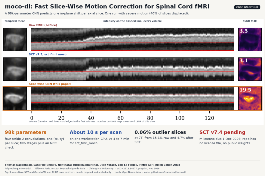
Spinal cord fMRI is one of the hardest scans to keep still. The cord sits next to the lungs, so every breath pushes it around, and patients shift their neck during a long run. The cord also does not move as one rigid block: one level can slide left while another stays put, and each thick axial slice is acquired at a different moment. The tool most labs use today, sct_fmri_moco in the Spinal Cord Toolbox (SCT), corrects this slice by slice with ANTs and takes 4 to 7 minutes per time series. A group from Polytechnique Montréal, Télécom Paris and Chiang Mai University has replaced that step with a convolutional network of about 98,000 parameters that does the same job in roughly 10 seconds on a CPU. The paper is arXiv:2611.14677, the code sits in the ivadomed/moco-dl repository, and the authors say the method ships in SCT v7.4.
What the method does
The task is narrow on purpose. For every axial slice of every volume in a 4D fMRI series, the network looks at two images stacked as channels: the slice to correct and a reference slice, by default the temporal mean of the series at that level. It outputs two numbers, the in-plane translation (tx, ty) that lines the slice up with the reference. Rotation, deformation and through-plane motion are left alone. Spinal cord pipelines have corrected motion with in-plane transforms per slice for years, and the restriction keeps the model tiny.
The architecture is four 3×3 convolutions with stride 2 and LeakyReLU (16 to 128 channels), an adaptive average pool and one linear layer. Before the network sees anything, a cropping step (sc-crop) finds the cord on the first volume and crops the same box around it for all volumes, which drops background tissue that moves differently from the cord and speeds up inference. Each slice is padded or cropped to 64×64 pixels, and intensities are clipped to the 1st to 99th percentiles and rescaled to [0, 1].
How it learns without motion labels
Real fMRI comes with no ground-truth motion, so the authors train the network to make the warped slice match the reference. The loss is normalized cross-correlation (NCC) between the corrected slice and the series mean. There are two models with the same architecture:
- M1 handles large, persistent movements. During training, each series gets a synthetic random walk added to it, independently along x and y, with steps drawn from a normal distribution and clipped to 3 voxels, so the fake motion drifts and persists the way real motion does. Its loss mixes a global NCC, which still gives a useful gradient when a slice is far off, with a local NCC over 5×5 windows that is sensitive to sub-voxel misalignment.
- M2 handles the small residual motion. It trains on the real series with no synthetic motion and uses the local NCC only.
Training uses five public OpenNeuro datasets with 141 subjects (133 at 3T, 8 at 7T), slices 1 to 5 mm thick, about 2.6 million training slice pairs. Each model trains in about 13 hours on one NVIDIA RTX PRO 6000.
At inference, M1 predicts a translation for every slice. A check then compares NCC before and after, and any translation that makes the match worse is replaced by no shift. M2 then refines the result up to six times, recomputing the reference mean from the corrected series each round and applying the same check. The transforms are composed and applied once to the raw, uncropped data, so the image is resampled a single time.
What they tested it on
Testing uses two public datasets that the model never saw in training. ds008784 has 120 runs from 40 healthy subjects at 3T (1.25×1.25 mm in-plane, 4 to 5 mm slices). ds007067 has 59 runs from 14 subjects at 7T (0.75×0.75 mm in-plane, 3 mm slices). The baselines are sct_fmri_moco from SCT v7.3, a slice-wise AFNI variant that follows the Neptune toolbox, and FSL FLIRT run slice by slice with a cord mask, which also estimates in-plane rotation.
With no ground truth, the paper scores four things inside a cord mask: temporal SNR (tSNR), DVARS (how much the signal jumps between consecutive volumes), a sharpness measure on the temporal mean, and the share of “outlier” slices whose cord is still displaced by more than one voxel. On the 7T set, the raw data had 15.6% outlier slices. sct_fmri_moco brought that to 4.7%, the network to 0.06%. At 3T the network had the best tSNR and DVARS of all four methods and took 10.4 seconds per scan against 251.8 seconds for SCT, measured on the CPU of one workstation without file input and output. FLIRT kept slightly sharper images at 3T (0.173 against 0.170), which the authors put down to its rotation estimate, and at 7T the slice-wise AFNI variant matched the network’s tSNR and outlier rate, with slightly better DVARS and sharpness, while being about three times slower.
What it does to a scan
Fig. 3 of the paper, which we used for the featured image, shows one 3T run with severe motion where 40% of the slices are displaced. Around volume 37 the cord jumps by several voxels. The figure plots the intensity along one line through the cord for every volume; red lines mark the cord edges in the first volumes. In the raw data the cord walks out of those lines and stays out. After sct_fmri_moco it is still out. After the network it sits inside the lines for the whole run, and the tSNR in the cord for that slice goes from 3.5 in the raw data to 19.5. A motion step has to catch a jump like this one; if it misses, every volume after volume 37 is compared against the wrong voxels.
Why a viewer or clinic team should care
Spinal cord fMRI is still mostly a research scan, so the people who should look at this are the teams that build the platforms where those studies get processed.
The runtime changes where the step can live. A correction that takes 4 to 7 minutes per series is a batch job. One that takes about 10 seconds on a workstation CPU, with no GPU, can run when a study arrives, and a QC view can show the corrected series next to the raw one.
The output is easy to audit. The model’s whole answer is two translations per slice per volume. A viewer can plot them over time, flag the volumes where the shift jumps, and let a physicist decide whether a run is usable, which is much easier than inspecting a dense deformation field.
The recipe also carries over to other slice-wise steps: a small network trained without labels on public data, plus an explicit check that rejects predictions that make things worse. The authors plan to apply it to spinal cord diffusion MRI next. If you build DICOM tooling for research sites, plan for the input side: SCT and this code read NIfTI, so a DICOM-to-NIfTI conversion sits in front of it.
We covered a different take on motion earlier with EventMC, a training-free motion correction method for 3D brain MRI, where the head moves as one rigid block.
What it does not tell you yet
- No ground truth. All methods align to the temporal mean, so the metrics measure temporal consistency, not anatomical accuracy, and interpolation alone changes them. The authors note that simulated motion of known amplitude would measure accuracy directly; the paper does not include that test.
- Translation only. The model cannot correct in-plane rotation or through-plane motion. FLIRT, which estimates rotation, kept slightly sharper images at 3T.
- Two test sets. One 3T dataset of healthy subjects and one 7T dataset, in a 4-page paper. The authors write that more extensive tests are warranted, and the paper reports no patient cohort.
- Release state. As of 13 November 2026 the latest SCT release is 7.3, which has an older experimental
-dloption forsct_fmri_mocobased on a DenseNet model with a disclaimer that it is not thoroughly validated. The 7.4 milestone on GitHub is due on 1 December 2026. The new model’s code is on thetd/25-inferencebranch of the repository, which has no license file and no published weights that we could find.
How to try it
If you already run SCT, wait for v7.4 and compare the new correction against sct_fmri_moco on a few of your own runs. To read the code now, clone ivadomed/moco-dl and check out the td/25-inference branch: the fmri folder has the network (rigid_model_translation.py), the two training scripts and infer.py. The script loads two checkpoints you supply, runs on CPU and writes the corrected NIfTI. Its defaults (three stage-2 iterations, nearest-neighbour interpolation) differ from the paper’s six iterations and bilinear setting, so change them if you want to reproduce the tables. The main branch still holds the older DenseNet version. Both test datasets are public on OpenNeuro.
Licensing comes in two parts. SCT is released under LGPL-3.0. The moco-dl repository has no license, which by default gives you no right to reuse the code in a product, so ask the authors before you copy anything out of it. Once the model ships inside SCT, SCT’s license should apply to it.
Source and license
Paper: Thomas Dagonneau, Sandrine Bédard, Nontharat Tucksinapinunchai, Uten Yarach, Loïc Le Folgoc, Pietro Gori and Julien Cohen-Adad, “Fast Slice-Wise Deep Learning Motion Correction for Spinal Cord Functional MRI”, arXiv:2611.14677 (cs.CV, 10 November 2026), a 4-page preprint with no venue stated. Affiliations: Polytechnique Montréal (Montréal, Canada); Télécom Paris, Institut Polytechnique de Paris (Palaiseau, France); Faculty of Associated Medical Sciences, Chiang Mai University (Chiang Mai, Thailand). Code: github.com/ivadomed/moco-dl, no license file. Toolbox: Spinal Cord Toolbox, LGPL-3.0. Data: OpenNeuro ds008784 and ds007067 for testing, five other OpenNeuro datasets for training, under their own terms. Featured image: Fig. 3 of the paper, Raw, SCT and proposed-method rows, panels cropped and scaled only.