
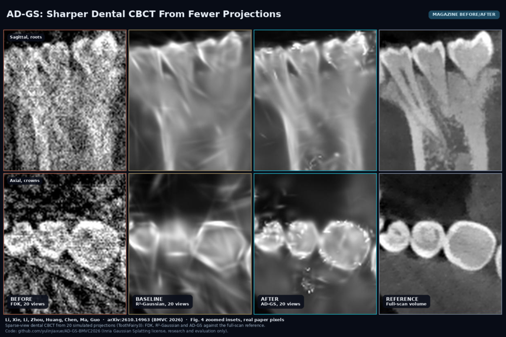
Every projection a dental CBCT scanner fires adds dose, so a short scan with fewer views cuts both dose and the chance of motion blur. Open the volume and you see what it costs. Reconstruct 20 or 30 projections with FDK, the filtered backprojection most scanners still use, and the tooth roots dissolve into streaks and grain. Zonglin Li, Kexian Xie, Feiran Li, Chu Zhou, Yixing Huang, Ruiyang Chen, Zhanyu Ma and Heng Guo (Beijing University of Posts and Telecommunications, Peking University Third Hospital, National Institute of Informatics in Tokyo and Peking University) posted arXiv:2610.14963 on 10 October 2026, a BMVC 2026 paper called AD-GS. It rebuilds a dental CBCT volume from sparse projections with 3D Gaussian splatting and spends most of its detail budget on enamel and bone. The code is public as yulinjiaxue/AD-GS-BMVC2026, under the Inria Gaussian Splatting license, which allows research and evaluation only.
Why a viewer team should care
Most dental software we build never touches raw projections. The scanner reconstructs, exports a DICOM series, and the viewer takes it from there: panoramic curves, cross-sections along the arch, canal tracing, implant planning, tooth segmentation. All of that inherits whatever the reconstruction did. If the roots are smeared, the automatic tooth segmentation is wrong, the canal overlay drifts, and the clinician is measuring blur. AD-GS sits one step upstream of the viewer, so it matters to you if you work with a scanner vendor, a research site that keeps projections, or a low-dose protocol study. The paper also scores reconstruction by what happens to downstream tooth segmentation, which is a test any viewer team can copy.
What goes in and what comes out
Input is a set of cone-beam projections with their scanner geometry (angles, source and detector distances) in the R²-Gaussian data format: a meta_data.json, the training projections as NumPy arrays, and an FDK volume used to seed the first point cloud. Output is a 3D attenuation volume, 256 x 256 x 256 in the experiments, saved as vol_pred.npy. There is no trained network to download. Each scan is fitted from scratch, the way NeRF-style reconstruction works, so the method needs no paired training data. It does cost time. The authors report about 27 to 30 minutes per scan on an RTX 4090, against roughly 14 minutes for R²-Gaussian and under two seconds for FDK (Table 3).
How it works
The volume is a cloud of up to 500,000 3D Gaussians. Each one has a position, a shape, an orientation and a peak attenuation, and the attenuation at any point is the sum of the Gaussians around it. Rendering a projection means integrating that field along each X-ray, which matches how the detector records the scan, and fitting means adjusting the Gaussians until rendered projections match measured ones.
The first change is where new Gaussians go. Earlier Gaussian splatting methods for CT clone and split primitives wherever the rendering gradient is large. With 20 views the gradients from different angles disagree and partly cancel, so detail ends up in the wrong places or nowhere. AD-GS treats the Gaussians as samples in a Markov chain Monte Carlo birth and death process, borrowed from 3DGS-MCMC: primitives that contribute almost nothing get moved, and the probability of landing near an existing Gaussian rises with its attenuation. Enamel, cortical bone and the thin gaps between teeth are small and dense, so they collect more primitives.
The second change is a structural loss. After about 20,000 of the 30,000 iterations, rendered and measured projections both go through a frozen MedSAM encoder (the repo loads MedSAM2). The 352-channel features are compressed to 16 with PCA, and the loss penalizes the cosine distance between them. The encoder is used zero-shot, with no labels and no fine-tuning. The features respond to boundaries and connectivity more than to raw intensity, so a tooth that splits or two teeth that merge cost more than a small intensity error. Total variation and an isotropy term keep the Gaussians from turning into needles that explain a few projections and nothing else.
What the numbers say
The authors ran an off-the-shelf tooth segmentation model, ToothSeg, on each reconstruction and scored the tooth masks for overlap, boundary agreement, connectivity and surface distance. At 20 views, tooth Dice is 88.3 percent for AD-GS, 78.8 percent for R²-Gaussian and 80.4 percent for FDK (Table 1). At 50 views the methods converge, with AD-GS and R²-Gaussian within half a point of each other, so the gain lives in the sparse regime. In the ablation, putting gradient-driven densification back in place of the density-guided placement costs a little on every metric at 20 and 30 views, while at 50 views the two are level. Dropping the MedSAM loss mostly hurts boundary agreement at 20 views.
The figure
The featured image uses the zoomed insets from Fig. 4 of the paper at 20 views: FDK, R²-Gaussian, AD-GS and the reference volume, a sagittal view of lower teeth and roots on top and an axial view of the crowns below. FDK is mostly grain. R²-Gaussian smooths the roots and crowns and leaves faint streaks across them. AD-GS keeps more of the root outlines and crown edges, and it also adds bright speckles along the enamel and in the soft tissue that are not in the reference. Check that speckle on your own data before you trust an automatic threshold on these volumes.
Limits
The evaluation is small and simulated. The team sampled 10 of the 37 ToothFairy3 scans, then generated 20, 30 and 50 projections from those already reconstructed volumes with TIGRE on a circular trajectory, adding Poisson and Gaussian noise. Real projections carry scatter, beam hardening, metal from fillings and implants, truncation and patient motion, and none of that is in the test. The reference is itself the clinical CBCT reconstruction of the full scan. The authors say the method still struggles below about 10 projections, and that it is tuned for hard tissue, so soft tissue and other body regions are untested. Thirty minutes per scan on a high-end GPU is fine for research and too slow for chairside use. The README’s checkpoint script and clone command still point to placeholder repositories, so you fetch the MedSAM2 weights yourself.
Code and license
The repository holds training, evaluation and visualization scripts, the vendored CUDA rasterizer from R²-Gaussian, and a minimal MedSAM2 fork for feature extraction. It is released under the Inria Gaussian Splatting license, which grants use for research and evaluation and forbids commercial use without the licensors’ consent. No patient data or trained reconstructions are bundled; ToothFairy3 comes from the challenge page under its own terms. For a product, evaluate the method with this code, then reimplement it or get the licensors’ consent before anything ships.
How we would wire it into a viewer
We would keep it outside the viewer, as an offline reconstruction job next to the scanner’s own recon. Take the projections and geometry from the vendor export, fit AD-GS on a GPU worker, convert vol_pred.npy back to a DICOM series with the original geometry and a new series description that says how it was made, and store it beside the vendor reconstruction instead of replacing it. In the viewer, hang both series with linked cursors so a clinician can flip between them on the same root or canal. Run your tooth segmentation on both and flag cases where the masks disagree by more than a set margin, which gives you a cheap QA signal. For background on the viewer side, see how to open a CBCT scan and CBCT arch cross-sections and panoramic rebuilds.
Sources
- Li, Z., Xie, K., Li, F., Zhou, C., Huang, Y., Chen, R., Ma, Z., Guo, H. AD-GS: Anatomical Density-guided 3D Gaussian Splatting for Sparse-View Dental CBCT Reconstruction. BMVC 2026. arXiv:2610.14963. https://arxiv.org/abs/2610.14963. PDF: https://arxiv.org/pdf/2610.14963.
- Code (Inria Gaussian Splatting license, research and evaluation only): https://github.com/yulinjiaxue/AD-GS-BMVC2026.
- Baseline and data format: R²-Gaussian (Zha et al., NeurIPS 2024), https://github.com/Ruyi-Zha/r2_gaussian. Dataset: ToothFairy3, https://toothfairy3.grand-challenge.org/.
- Featured image: zoomed insets from Fig. 4 of arXiv:2610.14963 (20 views; FDK, R²-Gaussian, AD-GS, reference), real paper pixels.