
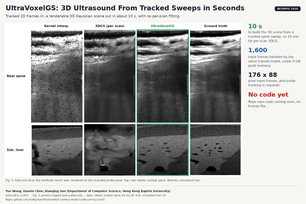
Freehand 2D ultrasound is still how most abdominal, vascular and musculoskeletal scans get done, and the sonographer builds the 3D picture in their head. Nobody sees which part of the organ was never swept until the patient has left. A group at Hong Kong Baptist University wants to change that with a live 3D view that keeps up with the probe. Yue Wang, Haoxin Chen and Xiaoqing Guo built UltraVoxelGS, a network that turns a sequence of tracked 2D ultrasound frames into a renderable 3D Gaussian scene in about 10 seconds, with no per-scan training. The paper is arXiv:2611.11951 and is accepted at NeurIPS 2026.
UltraVoxelGS is feed-forward. Earlier neural ultrasound reconstructions such as UltraNeRF, ImplicitVol or Gaussian splatting fitted to one scan optimize a fresh model for every patient, which takes minutes. UltraVoxelGS predicts the whole scene in one pass of an already trained network.
What UltraVoxelGS does
The input is what a tracked ultrasound system already records: 2D B-mode frames, each with a probe pose from an optical tracker, an electromagnetic tracker or a robot arm. The output is a cloud of 3D Gaussians that you can slice at any probe position and angle, including ones the operator never held.
Feed-forward Gaussian methods from photography do not transfer, and the paper explains why. They assume many overlapping photos of the same surface that look alike from different angles. Two ultrasound frames share at most a line, and the same tissue looks different depending on where the sound comes from, because echoes are direction-dependent and the signal fades with depth. So UltraVoxelGS works in two steps.
First, it uses the poses to place every pixel of every frame in 3D and blends them into one fixed voxel grid (0.75 mm spacing in the paper). This is close to classic freehand compounding. Then a Transformer reads small 8 × 8 × 8 voxel patches and predicts Gaussians for them. It only predicts the thin slab of the grid around each frame, then averages Gaussians where slabs overlap. Because the network sees the grid and not the raw frames, the cost depends on the volume size rather than on the number of frames.
Each Gaussian stores a direction-dependent echo strength and an attenuation value. The renderer multiplies the echo by how much signal survives along the beam path, so a structure under a strong reflector can appear darker, as it does on a real scanner. Nobody labels attenuation. It is learned only by matching rendered frames to recorded ones.
The last piece is Render-time Appearance Adaptation. When you ask for a view, the method finds the recorded frame whose probe center is closest, briefly adjusts the appearance values (not the geometry) so the render matches that neighbour, renders, and throws the adjustment away. This step does most of the sharpening. Without it, the rendered slices look smoothed by the voxel grid.
What they found
The main real dataset is a public set of robot-held lumbar spine sweeps with probe tracking from 63 healthy volunteers, with over 3,000 frames per scan. The second is 100 simulated liver sweeps generated from abdominal CT volumes in 3D-IRCADb and CRLM-CT. The test is held-out frames: the method never sees them, and the render at that pose is compared with the recorded image.
Building the scene takes 10.04 seconds per spine case, against 10 minutes for per-scan Gaussian splatting (3DGS) and 15 to 18 minutes for UltraGauss and UltraNeRF. On the spine data UltraVoxelGS also renders the held-out frames best, with a PSNR of 24.29 dB against 22.55 dB for 3DGS. On the simulated liver it is ahead on PSNR and SSIM but not on LPIPS, where UltraNeRF scores better.
The same trained model handles about 300, 600 or 1,600 input frames without retraining, and peak memory stays under 4 GB. On the paired handheld sweeps from the same spine dataset, again without retraining, it stayed close to its robot-held score (23.96 against 24.29 dB). When the authors added large synthetic tracking errors (about 21 mm and 10 degrees RMS), quality dropped by about 1.4 dB, mostly because the wrong neighbour frame got picked for the appearance step. A streaming mode updates only the blocks touched by each new group of 10 frames and comes out almost identical to reconstructing the whole sweep at once.
Why a viewer or clinic team should care
If you build ultrasound software, coverage feedback is the obvious first use. The Gaussians only carry evidence where frames passed. In the failure-case figure, under very sparse coverage, ImplicitVol and UltraNeRF return dense but smeared or noisy texture, while UltraVoxelGS leaves the under-covered region visibly incomplete. For a coverage display, that is the behaviour you want, because the hole tells the operator where to go back.
Review after the exam is the next use. A 10-second reconstruction can run while the patient gets dressed, and the radiologist can then reslice the sweep along planes that were never acquired. The appendix contrasts this with commercial compounding, which averages every revisit into one isotropic voxel value and so favors slow, even sweeps. Keeping direction-dependent echoes means the operator can scan a spot from a second angle to see past a shadow, and the model keeps both views.
The output is an explicit set of Gaussians, which is easier to store and send than a neural field, though it needs a renderer that knows the attenuation model. Rendering one slice without the appearance step takes 3.6 ms. With the default 50 adaptation steps it is 623 ms, fine for review but not for a 30 fps live view.
What it does not tell you yet
- It needs tracked frames. Without a tracker or a robot, you first need pose estimation from the images, and the paper does not test that.
- Low resolution. Frames go in at 176 × 88 pixels, far below what a clinical display shows. The paper does not report results at native resolution.
- Image quality, not diagnosis. Every number scores how well held-out frames are rendered, plus a SAM2-based liver segmentation check on the simulated data. Nothing measures whether a reader finds more or misses less.
- Narrow anatomy. One real anatomy (lumbar spine in healthy volunteers) and one simulated organ. No patients with pathology, no cardiac motion, no breathing.
- Hardware is unclear. The rendering timings were averaged across three V100 GPUs. The paper does not say what GPU produced the 10-second build, and training used one NVIDIA H20 for 300k iterations.
- Simplified physics. The renderer models reflection and attenuation only. Speed-of-sound changes, refraction, speckle decorrelation and vendor post-processing are not modelled, as the authors state.
How to try it
Not yet. The repository YuebyYue/UltraVoxelGS-camera-ready currently holds a README that says “Code coming soon”, a citation, and no license file. Watch it if you want to test it on your own tracked sweeps. The spine dataset (Cavalcanti et al., Scientific Data 2025) is public under CC BY 4.0, so a team with a tracked probe can at least compare its own compounding against the figures in the paper.
For a related idea on the CT side, see our post on CTBakeGS, which turns CT volumes into shareable Gaussian splat renderings. If your probe has no tracker, our post on estimating a six-DoF pose for untracked 2D ultrasound covers that missing step.
Source and license
Paper: Yue Wang, Haoxin Chen and Xiaoqing Guo, “UltraVoxelGS: Voxel-First Feed-Forward Gaussian Splatting for 3D Ultrasound Reconstruction”, Department of Computer Science, Hong Kong Baptist University, arXiv:2611.11951 (cs.CV, 9 November 2026), NeurIPS 2026. Code: github.com/YuebyYue/UltraVoxelGS-camera-ready, not yet released and with no license stated. Datasets: lumbar spine ultrasound from Cavalcanti et al. (CC BY 4.0); simulated liver sweeps built from 3D-IRCADb (CC BY-NC-ND 4.0) and CRLM-CT (CC BY 4.0) with the LOTUS simulator. Featured image: Fig. 5 of the paper, panels cropped and scaled.