
A 2D denoiser or super-resolution network restores one slice at a time, so it never sees the slice above or below the one it is fixing. A team from Kunming University of Science and Technology, Xi’an Jiaotong-Liverpool University, Massachusetts General Hospital and Harvard Medical School, and the University of Science and Technology of China (co-first authors Jialei He and Enhe Liu, corresponding authors Jiaman Ding, S. Kevin Zhou and Jinfeng Wang, 13 authors in total) posted arXiv:2610.12337 on 8 October 2026 with ContiLNN. It keeps an existing 2D restoration network and adds small bidirectional liquid neural network modules that pass information along the slice axis, and each step is told how many slice indices separate it from the previous slice it saw. The authors tested it on low-dose CT denoising, MRI super-resolution and low-count PET. Code, configs, evaluation scripts and six pretrained checkpoints are public on GitHub under Apache-2.0.
What goes in and what comes out
The input is a window of up to seven ordered low-quality 2D slices from one scan, together with their original slice indices. The output is one restored slice for every input slice, at the same positions. A whole series is covered by overlapping windows with two tiling offsets, and each slice’s final output is the average of the windows that contain it.
The indices are what make missing slices visible to the model. If only slices 1, 3, 5 and 7 survive, the gaps are 2, 2, 2. If slices 1, 2, 3, 5 and 6 survive, the gaps are 1, 1, 2, 1. The model receives those gaps as an input alongside the pixels.
Three tasks were tested, all on preprocessed benchmarks that come from the Restore-RWKV repository:
- CT denoising: quarter-dose in, normal-dose reference, from the AAPM Low Dose CT Grand Challenge. Eight patients for training, one for validation and one for testing (211 test slices).
- MRI super-resolution: IXI T2-weighted brain images, with the low-quality input made by keeping the central 6.25% of 2D k-space, which is four-fold along each in-plane axis. The slice axis is left as acquired. 114 test subjects.
- PET restoration: 159 scans from a PolarStar m660 system, with reduced-count inputs generated from list-mode data at a reduction factor of 12. 120 scans for training, ten for validation and 29 for testing.
How it works
The main backbone is Restore-RWKV, a 2D restoration network. Every slice still goes through its in-plane blocks unchanged. At selected levels of the feature hierarchy (intermediate encoder and decoder blocks, two skip connections, the bottleneck and the final refinement path, 16 modules in the Restore-RWKV setup), ContiLNN lines up the feature vectors at each in-plane location as a short sequence over the slices in the window. A forward cell runs through that sequence from first slice to last, a backward cell runs from last to first, and a linear projection fuses the two states at each slice position. Most insertion points add this result back through a learnable gate, so training decides how much slice context to mix in. The bottleneck runs it in series before the decoder.
Each cell is a closed-form continuous-time (CfC) unit, a member of the liquid neural network family from Hasani and colleagues. The new state is a per-channel blend of two candidate states, and the blend weight depends on the current slice’s features, the incoming state and the slice gap divided by the window size. A larger gap can shift that blend, and different channels can react in opposite directions. The update is a direct formula, so there is no ODE solver and no iteration per step.
Training starts from the best checkpoint of the plain 2D backbone and uses three losses. An L1 reconstruction loss compares each restored slice with its high-quality reference. A cross-slice consistency loss compares the first and second differences between successive slices in the output with the same differences in the reference, which penalizes error that changes from slice to slice while keeping the real anatomical change. A distillation loss keeps each output close to what a frozen copy of the pretrained 2D backbone predicts for that slice alone. The frozen copy is only used during training.
What the numbers say
Averaged over five training seeds, ContiLNN on top of Restore-RWKV raises mean PSNR over the per-slice Restore-RWKV baseline by 1.02 dB for MRI super-resolution (32.07 to 33.08 dB) and 1.25 dB for PET (37.27 to 38.52 dB), with higher SSIM and lower RMSE in both (Table 1). In the case-level analysis, all 114 MRI subjects and all 29 PET scans improve on PSNR, SSIM and RMSE, with median PSNR gains of 1.04 dB and 1.17 dB (Fig. 6). The CT gain is 0.19 dB (33.76 to 33.95 dB), and it comes from one held-out patient. The 0.0026 dB spread across seeds shows that training repeats well on that patient. It says nothing about how the gain varies between patients, and the authors state this themselves.
The idea also transfers to a second backbone. On DASMamba, PSNR rises by 0.19, 0.36 and 1.13 dB for CT, MRI and PET, though SSIM drops slightly for CT and MRI (by 0.0051 and 0.0050).
For anyone sizing hardware, Table 4 is the useful one. It is measured at 128 x 128 pixels, 32-bit precision, on one NVIDIA A800, with a seven-slice window. The Bi-CfC modules add 6.56 million parameters and 22.88 GMACs per slice to Restore-RWKV. Median forward time per slice goes from 16.72 to 25.69 ms, and peak memory from 987 to 995 MB. A bidirectional GRU in the same slots, with nearly the same parameter count and compute, takes 54.42 ms per slice and 2,316 MB, and restores slightly worse (38.52 vs 38.59 dB PSNR on PET).
The context test in Table 6 shows that the model uses its neighbors. With the same PET checkpoint, reversing the slice order costs 0.26 dB, feeding the center slice seven times costs 2.62 dB, and feeding unrelated slices from the same patient costs 6.35 dB.
What the pictures show
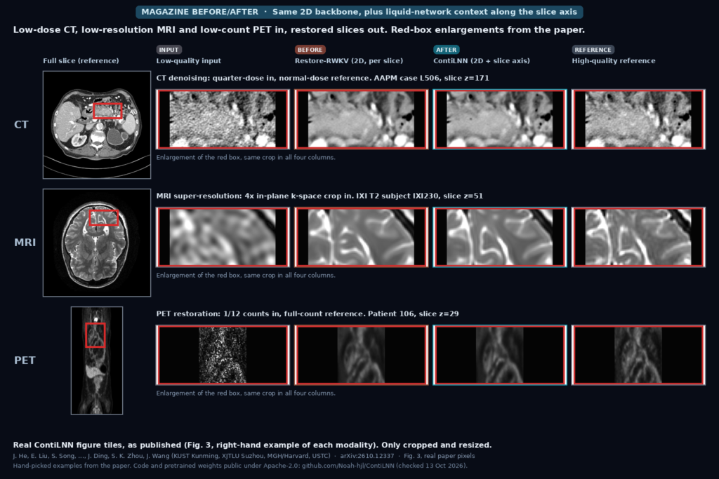
The featured image is cut from Fig. 3 of the paper, the right-hand example for each modality: CT case L506 at slice 171, IXI subject 230 at slice 51, and PET patient 106 at slice 29. On the left is the full reference slice with the authors’ red box. To its right are the enlargements of that box for the low-quality input, the per-slice Restore-RWKV output, the ContiLNN output and the high-quality reference.
The input columns show the degradation clearly: grain in the CT, blur in the MRI, speckle in the low-count PET. At banner size the Restore-RWKV and ContiLNN columns look close to each other, which fits a 0.19 dB CT gain and a roughly 1 dB MRI gain. The paper shows the differences in two other places. Its error-reduction maps (the fifth column of Fig. 3, not in the banner) put the larger reductions at tissue interfaces. Its seven-slice intensity profiles (Fig. 4) show ContiLNN tracking the reference through peaks and drops along the slice axis, with mean absolute deviation falling from 0.290 to 0.135 at one CT location, 0.150 to 0.066 at one MRI location and 0.257 to 0.085 at one PET location. These are hand-picked locations from the paper.
Where it falls short
The gaps are counted in slice indices. The preprocessed benchmark data carried no physical slice spacing, so the model has never seen a real DICOM slice position or spacing value. The authors list physical coordinates from DICOM metadata as future work. A series with uneven spacing would have to be mapped onto an index grid before this model could use it.
Missing slices still cost quality unless you train for them. The main model is trained on contiguous windows. On the PET test set it drops 1.92 dB when only every third slice is present (to 36.67 dB), which is below the 37.27 dB that per-slice Restore-RWKV gets on the same cohort. Training on mixed gaps of 1, 2 and 3 brings that case up to 38.00 dB, and after mixed-gap training a bidirectional GRU matches or slightly beats Bi-CfC on PSNR at uniform gaps (Supplementary Table S5). Bi-CfC still wins on irregular gaps and on memory and speed.
The evaluation is narrow. CT has one test patient. Each modality comes from one source: one public CT challenge, one public MRI collection with simulated k-space truncation, and one PET scanner model. Generalization across protocols has not been tested, and there is no reader study or downstream task such as detection or segmentation. Quality is reported only as PSNR, SSIM and RMSE. The slice modules also add parameters and about 54% to per-slice forward time over the 2D backbone.
Code, weights, and data
The repository is github.com/Noah-hjl/ContiLNN, under the Apache License 2.0. Restore-RWKV files keep their upstream Shanghai AI Laboratory notice, and DASMamba is a pinned external dependency. When I checked on 13 October 2026, the release pretrained-v1 held six checkpoints of about 140 MB each: ContiLNN-RWKV and ContiLNN-DASMamba for CT, MRI and PET. The contilnn command covers protocol inspection, training from a 2D backbone checkpoint, and case-level evaluation that writes per-slice and per-case CSV files. CPU tests run without data or weights.
No imaging data ships with the code. The readers expect per-slice files (pickled .bin arrays or NIfTI) in a fixed folder layout with modality-specific filename patterns, and there is no DICOM reader. The README warns that checkpoints and .bin files are deserialized with PyTorch and pickle, so only load files from sources you trust. The Restore-RWKV WKV CUDA extension compiles on first run, and the DASMamba variant needs mamba-ssm and the pinned DASMamba source.
How we would wire it into a viewer
We would run it as a server-side job that writes a new derived series and never replaces the original. Read the series, sort the slices by their position along the slice normal, convert positions to an index grid (and flag the series if spacing is uneven), restore in overlapping seven-slice windows, and write the result as a new series with its own Series Instance UID, ImageType DERIVED\SECONDARY and a derivation description that names the model and checkpoint. In the viewer it opens next to the source with synchronized scrolling and a clear “AI restored” label, so a reader can flip back to the acquired pixels at any time.
The public weights were trained on one CT challenge set, IXI T2 brains and one PET scanner, so we would treat them as a starting point and fine-tune on our own sites’ paired data. If our series often arrive with missing slices, we would use the mixed-gap training recipe from the start. Before shipping, we would time it at our real matrix size (the paper profiles 128 x 128), run a no-reference quality check across sites, and have a reader compare small structures against the source. For related work on this site, see our posts on low-dose CT denoising without paired normal-dose training, a no-reference CT quality score and slice-consistent brain MRI inpainting.
Sources
- He, J., Liu, E., Song, S., Jin, P., Su, J., Wang, H., Lu, Z., Huang, Y., Cai, A., Jiang, Z., Ding, J., Zhou, S. K., Wang, J. ContiLNN: Mitigating Slice Sampling Discontinuity with Liquid Neural Networks for Medical Image Restoration. arXiv:2610.12337, 2026. https://arxiv.org/abs/2610.12337. PDF: https://arxiv.org/pdf/2610.12337.
- Code and pretrained weights: https://github.com/Noah-hjl/ContiLNN (Apache-2.0, release pretrained-v1, checked 13 October 2026).
- Hasani, R., Lechner, M., Amini, A., Liebenwein, L., Ray, A., Tschaikowski, M., Teschl, G., Rus, D. Closed-form continuous-time neural networks. Nature Machine Intelligence 4, 992 to 1003, 2022.
- Yang, Z. et al. Restore-RWKV: Efficient and effective medical image restoration with RWKV. IEEE Journal of Biomedical and Health Informatics, 2026. Chan, S. C. K. et al. Directional adaptive shuffle-based visual state-space models for medical image restoration (DASMamba). MICCAI 2025.
- McCollough, C. H. et al. AAPM Low Dose CT Grand Challenge (2017); IXI Project; PolarStar m660 PET cohort from Yang et al. (2024), as cited in the paper.
- Featured image: Fig. 3 of arXiv:2610.12337 (right-hand CT, MRI and PET examples with red-box enlargements), as published.