
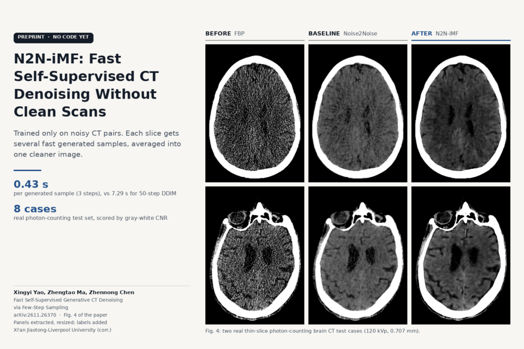
Thin-slice head CT, low-dose abdominal CT and the new photon-counting scanners all hand you the same problem: more grain than a reader wants, and no clean scan of the same patient to train a denoiser against. Xingyi Yao, Zhengtao Ma and Zhennong Chen (arXiv:2611.26370, preprint, 19 November 2026; corresponding author at Xi’an Jiaotong-Liverpool University) train a generative denoiser on noisy pairs only, then make it fast enough that averaging many generated samples per slice is practical. They call it N2N-iMF, Noise2Noise with Improved Mean Flow.
For head CT, the training pairs come from neighbouring reconstructed slices, so a site can build a training set from a DICOM export, with no raw projections and no matched normal-dose scans.
Why plain Noise2Noise looks waxy
Noise2Noise trains a network to predict one noisy image from another noisy image of the same anatomy. If the two noise realisations are independent and zero-mean, the squared-error optimum is the same as if you had trained on clean targets. Regression returns the conditional mean, and the mean of all plausible clean images is a smooth image. Small vessels and fine sulci fade along with the grain.
An earlier paper by Zhennong Chen and colleagues (SPIE Medical Imaging 2026) got around this by training a conditional diffusion model to generate the noisy partner image, then averaging several independent samples. Each sample keeps realistic texture, and averaging cancels the noise. Each sample needed a full multi-step diffusion run, and averaging needs ten or twenty samples per slice, so inference was slow.
What N2N-iMF changes
N2N-iMF swaps the diffusion generator for an Improved Mean Flow model. A mean flow network predicts the average velocity over a time interval along the generation path, which lets it go from Gaussian noise to an image in a few large steps. The network is a conditional U-Net that sees the noisy input and generates a plausible noisy partner. At inference you draw K independent samples, each in a handful of network evaluations, and average them. The noise in the samples is independent, so it shrinks with averaging, while the anatomy, which every sample agrees on, stays.
Training pairs are built two ways. For the simulated abdominal CT, each sinogram is split into two disjoint halves and reconstructed separately. For brain CT and photon-counting CT, the two neighbours of a slice are stacked as the input and the middle slice is the target. On those two datasets the authors also fine-tune with a PatchGAN loss so that local texture matches the noisy targets.
The number of averaged samples, K, works as a strength setting: one trained model gives lighter or heavier denoising depending on how many samples you average, with no retraining.
What the results show
The test data are 10 normal-dose cases from the AAPM Low Dose CT Grand Challenge with simulated low dose (seven for training, three for testing), 100 retrospective brain CT scans with simulated thin-slice noise (84 and 16), and 33 real portable photon-counting brain scans at 120 kVp, 6 to 7 mA and 0.707 mm slices (25 and 8).
With three network evaluations per sample and ten samples, N2N-iMF reached a mean absolute error of 2.60 HU on brain CT and 14.02 HU on abdominal CT, against 2.91 and 14.53 HU for DDIM with 50 evaluations per sample. One sample took 0.43 s on an RTX 4080 Laptop GPU, against 7.29 s for 50-step DDIM. On the eight real photon-counting cases, which have no clean reference, mean gray-white matter contrast-to-noise ratio was 1.341, against 0.916 for Noise2Noise and 1.176 for DDIM.
In Fig. 1, a supervised diffusion model trained on a different noise model and reconstruction kernel changes local texture on the abdominal case, while N2N-iMF, trained on the target data, keeps small vessels in the magnified inset. In Fig. 4, Noise2Noise output on photon-counting scans is smooth and flat, DDM2 leaves heavy residual noise, and N2N-iMF keeps the cortical sulci visible.
Where it would fit
This is a post-reconstruction filter: a CT series in, a denoised series of the same geometry out, which a viewer or PACS-side service can store as a derived series next to the original. The head CT recipe needs only reconstructed thin slices, so a site could train on its own scanner, kernel and dose protocol without a vendor’s raw data, the setting where Fig. 1 shows an off-the-shelf supervised model drifting. K maps onto a “denoise strength” control in a viewer.
The cost sits in the sampling. At three evaluations per sample and ten samples, a slice needs 30 network passes; by our multiplication of the paper’s per-sample time that is a little over 4 s per 512 x 512 slice on a laptop GPU at batch size 1, before any batching. The photon-counting setting used five evaluations and 20 samples, which is 100 passes per slice. A thin-slice head stack of several hundred slices would run as a background job after the series arrives.
Limits
- Small real-data test. The real photon-counting evaluation is eight cases with no low-noise reference, scored only by contrast-to-noise ratio in hand-drawn regions and visual inspection. There is no reader study and no check for missed or invented findings, which the authors name as their main limitation.
- Simulated noise elsewhere. Abdominal and brain results use Gaussian noise added in the projection domain, and the abdominal test set is three patients.
- Interpolated references. The “clean” thin-slice brain references are 5 mm volumes interpolated to 0.625 mm, so they are smoother than a true thin acquisition.
- Adjacent-slice assumption. Slice pairing assumes neighbouring slices show nearly the same anatomy. That holds for sub-millimetre head CT and gets weaker for thick slices or regions where anatomy changes quickly along the table.
- 2D, per slice. The network works on single 512 x 512 slices, with neighbours as context only.
- Generative output. Every sample is generated, and averaging reduces but does not remove sample-to-sample variation. A clinical product would need lesion-level validation before anyone reads from it.
Code and licence
The paper links no code or weights, and as of 21 November 2026 we found no N2N-iMF repository or model card. The corresponding author’s GitHub (zhennongchen) has code for the earlier diffusion Noise2Noise work (CTDenoising_Diffusion_N2N, Diffusion_denoising_thin_slice) and for the DDM2 and Noise2Score baselines, none with a licence file, which by default grants no reuse rights. The AAPM challenge data are public; the brain CT and photon-counting scans are institutional and not released.
For related reading on our side, see self-supervised low-dose CT denoising from a single scan, spectral decomposition for photon-counting CT and DuSS-PET for low-dose PET without paired data.
Source
Paper: Xingyi Yao, Zhengtao Ma and Zhennong Chen, “Fast Self-Supervised Generative CT Denoising via Few-Step Sampling”, arXiv:2611.26370 (v1 19 November 2026), preprint. Corresponding author: Zhennong Chen, Xi’an Jiaotong-Liverpool University. Featured image: Fig. 4 of the paper (two real thin-slice photon-counting brain CT cases: FBP, Noise2Noise and N2N-iMF), panels extracted from the PDF, resized, with labels added.