BasisSimulator.jl: One Spectral CT Decomposition for Every Scanner

If you build software that touches spectral CT, whether a virtual imaging trial, a reconstruction prototype or a research viewer that shows iodine maps, you have probably hit the same problem. Every scanner family ships its own material decomposition, nobody outside the vendor can see it, and the open methods you can find are usually written for one acquisition type. Dale Black, Surya Naidu, Hamidreza Khodajou-Chokami and Sabee Molloi of the Department of Radiological Sciences at the University of California, Irvine, posted a projection-domain method on 21 October 2026 in arXiv:2610.30440. The same estimator runs on rapid kVp-switching, dual-source and photon-counting data without being rewritten, and it ships in their open-source CT simulator.

Why a simulation or reconstruction team should care

Virtual imaging trials simulate several vendor systems on the same virtual phantoms and patients. If each simulated scanner gets its own decomposition code, part of the difference you measure between scanners comes from the code. The authors apply one estimator to all three simulated acquisitions, so the differences they report come from the acquisitions. For a photon-counting team the other draw is that you can keep every energy window instead of summing them down to two.

What the method does

Projection-domain decomposition takes the spectral measurements along each ray and estimates two basis line integrals, here iodine and water, before any reconstruction. That keeps beam hardening out of the images, and you reconstruct the two basis sinograms with ordinary filtered backprojection afterwards.

The starting point is the univariate method of Cong et al. from 2022. It expresses the water line integral as an odd-order polynomial of the iodine one, so a two-variable inversion becomes a one-variable search. The catch is that it is written for exactly two measurements made with two x-ray spectra. Photon-counting data with four energy windows has to be summed down to two before you can use it.

The new method keeps the idea of searching in one dimension but drops the polynomial. For a fixed iodine value, an inner Fisher-scoring loop finds the water value that minimizes the Poisson negative log-likelihood over all K measurements. An outer Fisher-scoring loop then moves the iodine value along that profile. Each measurement is described by its own spectral response, which includes the source, filtration and detector, so a kVp pair and a set of photon-counting windows enter the model in the same way. There are no regularization weights, no training data and no calibration tables. You do need to know the spectral response of each measurement.

What they found

The authors simulated three scanners: a GE Revolution Apex Elite with rapid switching between 80 and 140 kVp, a Siemens SOMATOM Definition Flash with dual-source 80 and Sn140 kVp, and a Siemens NAEOTOM Alpha photon-counting scanner at 140 kVp with four windows at 20, 35, 55 and 70 keV. Phantoms were the Gammex 472 and a tissue-characterization phantom.

• Accuracy on the line integrals. On noiseless data, the iodine error stayed below 3 × 10^-6 g/cm². On noisy data, the estimator noise came within 3% of the Cramér-Rao lower bound for a representative ray.
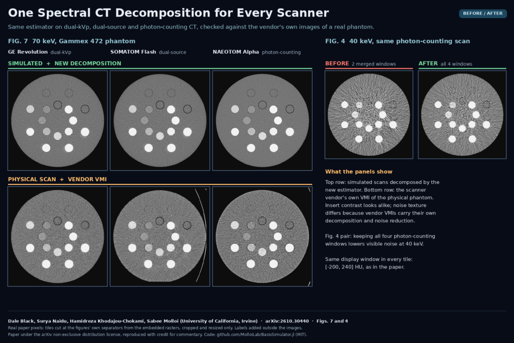
• Agreement with real scanners. The Gammex 472 was also scanned on all three physical systems. At 70 keV and above, VMIs from the simulation matched the vendor VMIs with a mean absolute error of 6 to 22 HU.
• Four windows beat two. On the photon-counting acquisition, keeping all four windows instead of summing them into two lowered the iodine bound by 19% and image noise by 8 to 16% at every VMI energy. The regression error at 70 keV dropped from 5.2 to 3.1 HU.
• Speed. 0.34 to 0.67 s per million rays on an NVIDIA A100, about 1.8 to 2.2 times the univariate method.
• Settings. Changing iteration limits and tolerances moved CT numbers by less than 0.04 HU.

The featured image shows Fig. 7 of the paper on the left. The top row is the simulation decomposed by the new method, the bottom row is the vendor VMI of the physical phantom on each scanner, all at 70 keV. Insert contrast looks alike. The noise texture differs because the vendor images carry the manufacturer’s own decomposition and noise reduction, which is why the authors compare CT numbers only. On the right is the 40 keV photon-counting tile from Fig. 4 with two merged windows and with all four.

The detector test

If you work on photon-counting data, read Section 3.5. With pile-up and scatter left in the counts and an ideal detector response, the estimator could not fit the data. With the same uncorrected counts and a response that included pile-up, charge sharing and escape, it recovered to within a few HU of the fully corrected result at 100 and 140 keV. Only scatter had to be corrected in the data. The detector enters the method only through its spectral response, so a good detector model replaces most of the count corrections in this simulation.

What this means for your stack

1. If you run virtual imaging trials across vendors, use one decomposition for every simulated system so the comparison isolates the hardware.
2. If you have photon-counting data with more than two windows, try the K-window estimator before you merge windows. The paper shows the merge costs noise.
3. Budget for the spectral model. The method is only as good as the response you give it, and the paper has not yet tested it on measured projections.
4. Treat low-energy calcium with care. At 40 keV the calcium error grew with four windows, which the authors trace to the water/iodine basis.

Where it falls short

• Simulation only. The estimator was never run on measured projection data. The physical scans were compared only through the vendors’ VMIs.
• Same model both ways. The simulated data were generated with the same spectral model used for decomposition, so spectral-model mismatch is untested.
• Two-material basis. Calcium at 40 keV went from 17.7 to 70.7 HU error with K = 4. A larger basis would be needed.
• Idealized geometry. Dual-energy rays were assumed co-registered, which real kVp-switching and dual-source systems do not provide directly. Electronic noise is not modeled.
• Narrow comparison. The baseline is the univariate method it generalizes, not a joint two-dimensional likelihood search. Deep-silicon detectors were not modeled.

Code and license

The estimator ships in BasisSimulator.jl, MIT licensed, Julia 1.12 or newer, on CUDA, Metal, ROCm, oneAPI or CPU. The K-channel decomposition and the VMI chain became package code in v0.15.0 (released 26 September 2026); the paper’s simulations used v0.14.0. There are no weights because nothing is trained. The paper itself is under the arXiv non-exclusive distribution license, and the authors disclose AI assistance for the manuscript and code.

Related reading on PYCAD

• AD-GS: Sharper Dental CBCT From Fewer Projections
• DeBoneDiT: Soft-Tissue Chest X-Rays Without Dual-Energy Hardware
• TB-PET-DDS: A Diffusion Prior for Low-Count Total-Body PET

Sources

• Dale Black, Surya Naidu, Hamidreza Khodajou-Chokami, Sabee Molloi. Unified Projection-Domain Material Decomposition for Energy-Integrating and Photon-Counting CT. arXiv:2610.30440, 2026. Abstract and PDF.
• Code: github.com/MolloiLab/BasisSimulator.jl (MIT). Documentation: molloilab.github.io/BasisSimulator.jl.
• Featured image: Figs. 7 and 4 of the paper, cropped and resized only.