
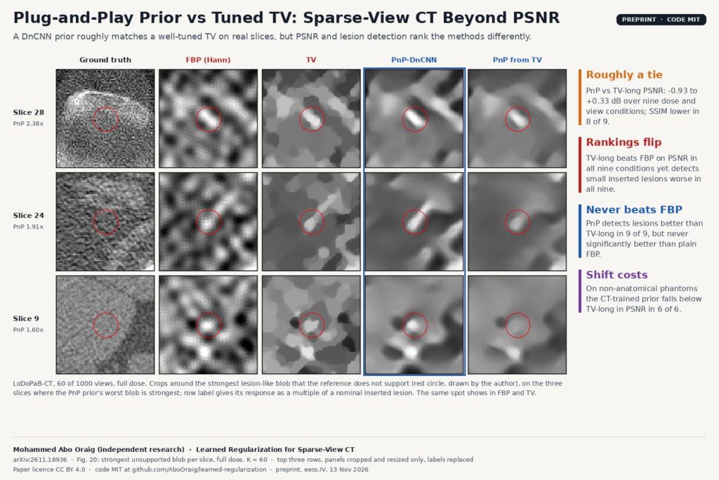
Papers that propose a learned CT reconstruction usually report PSNR and SSIM on test images that resemble the training set. A 62-page preprint by Mohammed Abo Oraig, arXiv:2611.18936 (eess.IV, 13 November 2026), takes one standard learned approach, a Plug-and-Play denoiser prior for sparse-view CT, and tests it against a tuned total-variation (TV) baseline on three questions: whether its advantage survives a change of image distribution, whether it invents lesion-like structure, and whether PSNR predicts if a small lesion stays visible. On real CT slices the learned prior roughly matches TV on PSNR, and PSNR and lesion detection disagree on which method is best. The protocol carries over to anyone who has to validate a reconstruction or denoising stage before it reaches a viewer.
What it does
The paper proposes no new method. The author takes a plain Plug-and-Play (PnP) scheme and compares it with filtered back-projection (FBP), Tikhonov and TV regularization, with every method tuned on held-out validation data for every condition and every comparison paired on the same images. The study runs first on 28 by 28 digit images, where noise, angle count, forward-model error and the prior’s training data can all be varied and repeated, and then on real 362 by 362 slices from the public LoDoPaB-CT dataset, whose ground truth derives from the LIDC-IDRI chest CT collection.
Besides PSNR and SSIM, every reconstruction is scored on a task. Small synthetic lesions are inserted into the slices, the slices are reconstructed, and a simple location-known observer measures whether the lesion can still be told apart from a lesion-free reconstruction (a paired AUC). The same observer counts lesion-like blobs that appear in lesion-free reconstructions where the reference image has none.
How it works
- The learned prior. A small DnCNN-style denoiser, 8 convolutional layers of 3 by 3 kernels with 64 channels, takes the noise level as a second input channel so one network covers every denoising strength. For the CT study it was trained on 8,960 LoDoPaB slices for 15,000 steps. A deeper 17-layer variant was also trained and did not help.
- The PnP loop. Each iteration takes a gradient step toward agreement with the measured sinogram, then passes the image through the denoiser in place of a hand-written regularizer. The loop starts from an FBP image, and both the denoising strength and the number of iterations are tuned. In the CT grid the tuned iteration count was at most 12; the paper shows that stopping early acts as part of the regularization.
- The classical baselines. FBP with a Hann window whose cut-off is tuned, and box-constrained TV solved with the Chambolle-Pock primal-dual algorithm for 150 iterations. A second TV run, TV-long, uses 300 iterations with its own tuned weight, to check whether TV only loses because it was given fewer iterations.
- The CT setting. Parallel-beam geometry with 1000 angles on 513 detector bins, subsampled to 30, 60 or 120 views. Doses of 1, 0.25 and 0.1 of 4,096 photons per detector bin are obtained by exact binomial thinning of the real counts. Tuning uses 20 validation slices from 20 patients, and evaluation uses 40 test slices, one per patient, from patients the prior never saw.
- The lesion test. Gaussian blobs with widths of 2 and 4 pixels (1.4 and 2.9 mm) and a contrast the author estimates at roughly 240 HU, four per slice, inside the body. These are small but not low-contrast lesions in the clinical sense.
What they found on real CT
On the 40 test patients, the learned prior does not consistently beat a well-tuned TV. Against TV-long, its PSNR difference ranges from minus 0.93 to plus 0.33 dB over the nine dose and view conditions, and its SSIM is lower in eight of nine. The roughly 3.4 dB advantage it had on digits at moderate noise does not carry over to clinical-size slices.
On lesion detection the PnP reconstruction detects the inserted lesions better than TV-long in all nine conditions, by 0.03 to 0.16 in AUC, significantly in six. But it is never significantly better than plain Hann-filtered FBP. TV-long, meanwhile, is 0.81 to 2.28 dB better than FBP in PSNR and has a lower detection AUC than FBP in all nine conditions, significantly in seven. PSNR and lesion detectability rank the three methods in opposite orders. At 60 views and full dose, the regularized methods keep only 7 to 32% of an inserted lesion’s local contrast, against 31 to 67% for FBP, so their detection scores come mainly from suppressing background noise.
In distribution, the prior invents little. The PnP reconstruction produces 0.24 to 1.38 lesion-like false blobs per slice in the four conditions tabulated, fewer than FBP in each of them. The featured image (Fig. 20 of the paper) shows the slices where the learned prior’s worst false blob is strongest, and in each row a bright spot sits at or near the same place in the FBP and TV reconstructions. The author reads these as coming from the data (few views, noise, streaks) and not from the prior, while noting a few prior-specific cases and that 40 slices with one noise draw cannot rule out rare ones.
Applied without retuning to 20 piecewise-constant phantoms, the CT-trained prior falls below TV-long in PSNR in all six conditions tested, and its detection advantage is significant in only one of six. On digits the shift effect was larger: an MNIST-trained prior went from beating TV to sitting 3.1 dB below it on Fashion-MNIST and 4.3 to 4.6 dB below it on the Shepp-Logan phantom, while a prior trained on Fashion-MNIST beat TV there, which points at prior mismatch rather than at PnP itself.
Why a viewer or clinic team should care
If you integrate a learned reconstruction or denoising step into a CT pipeline, or you are asked to sign off on one from a vendor, a PSNR or SSIM table is the number you will usually be handed. In this study that number ranked methods in the opposite order from a lesion-detection task on the same slices, and a prior that was far ahead on simple images was only on par with a tuned classical method on real anatomy.
The author lists practices for such studies, offered as suggestions rather than tested conclusions: give the classical baseline the same constraints and a tuned iteration count, tune every method on held-out data, train several seeds, test one matched and one mismatched prior, add a task-based metric next to PSNR and SSIM, and state the data model explicitly. A team with access to its own scanner data can run a version of the lesion-insertion test before a new reconstruction reaches the reading room. In a viewer, a side-by-side panel of FBP, TV and learned output on the same slice, with the inserted test lesions marked, lets a physicist or radiologist see these differences directly, as Fig. 20 does.
What it does not tell you yet
- It covers one small denoiser in one PnP scheme. End-to-end networks, unrolled methods, diffusion priors and commercial deep-learning reconstruction were not tested, and the author makes no claim about them.
- The CT geometry is 2D parallel-beam on LoDoPaB slices, with Poisson noise simulated on a finer grid. No fan-beam, cone-beam, helical or vendor raw data were used.
- LoDoPaB’s ground truth is itself a reconstruction, so a “false” blob means unsupported by that reference, not proven absent from the patient.
- The lesions are bright Gaussian blobs of roughly 120 to 240 HU under an assumed intensity mapping, the observer knows where they are, and no reader study was done. Low-contrast lesions, search tasks and human readers remain untested.
- Every operating point was tuned for PSNR, not for detection. A detection-tuned TV or PnP might rank differently.
- The CT study has one denoiser training run, one noise realisation per condition and 40 patients, so a single AUC cell is uncertain by about plus or minus 0.05.
- The analysis was developed in steps after seeing results, with no pre-specified primary comparison and no multiplicity correction. The author documents each step, including an early comparison that was discarded.
- The shift test on real CT uses piecewise-constant phantoms chosen to favour TV. A change of scanner, protocol or anatomy was not tested.
How to try it
The code is public at github.com/AboOraig/learned-regularization under the MIT licence, with the trained digit and CT denoiser weights, raw per-image results, figure scripts and 68 unit tests. The CT experiments need the LoDoPaB-CT files from Zenodo; a synthetic smoke test runs without any download. The author discloses that an AI assistant helped with the code, the experimental design and the editing. On the blog, see also LesionStudio, tuning PET and SPECT reconstruction with synthetic lesions, EUReCA for sparse-view linac CBCT and why a no-reference quality score should not pick your CT denoiser.
Source and license
Paper: Mohammed Abo Oraig, “Learned Regularization for Sparse-View CT: Accuracy, Lesion Detectability and Distribution Shift of a Plug-and-Play Prior against Tuned Total Variation”, arXiv:2611.18936 (eess.IV, 13 November 2026), preprint, not peer-reviewed, 62 pages; also on Zenodo (doi:10.5281/zenodo.24107061). Affiliation: independent research. Paper licence: CC BY 4.0. Code and weights: MIT. Data: LoDoPaB-CT, derived from LIDC-IDRI. Featured image: Fig. 20 of the paper, three rows cropped and resized only.