
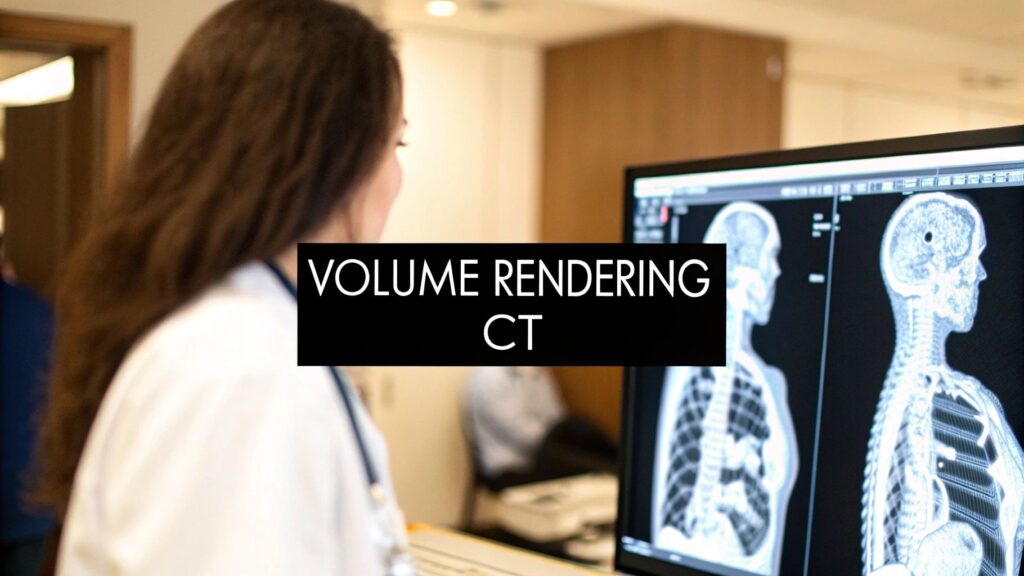
Volume rendering of CT paints every voxel in a scan — not just a surface — so you can see vessels, bone, and soft tissue in one 3D view. The useful knobs are MIP vs DVR, transfer functions, and (when you want film lighting) cinematic rendering. This page is that visualization. It is not how the scanner acquired the volume, and it is not a VTK mapper how-to.
If you meant volumetric / helical acquisition → what a volumetric CT scan is. If you meant GPU / VTK rendering → GPU volume rendering for faster CT visualization. If you meant reconstruction (FBP / IR) → 3D reconstruction from CT. If you meant 3D imaging software to buy → 3D imaging software. If you meant a printable mesh → CT scan to 3D model / DICOM to STL.
From slices to a volume
A CT is a stack of 2D slices. Volume rendering treats that stack as a 3D grid of voxels. Each voxel holds a density (Hounsfield units). The renderer walks rays through the grid and decides, per sample, how much color and opacity that density should contribute. Rotate the camera and you are not flipping a photograph — you are re-casting the same volume.
That only looks good when the voxels are close to cubes. MDCT made isotropic (or near-isotropic) volumes routine: same size in x, y, and z, so a coronal or sagittal reformat is not a smear. The scan mode that produces that volume is volumetric CT. This page starts after the volume exists.
MIP vs DVR
| Technique | What it does | Best for | Cost |
|---|---|---|---|
| Maximum intensity projection (MIP) | Keeps the brightest sample along each ray | Vessels, contrast, bone — anything that should “glow” | Cheap. Hides what sits behind the bright voxel |
| Direct volume rendering (DVR) | Composites color + opacity along the ray | Soft tissue, organs, mixed anatomy | Needs a transfer function. Heavier than MIP |
MIP is a projection, not a shaded scene. A bright stent or contrast bolus can erase the vessel behind it. DVR is the “see through the volume” picture people mean by volume rendering. Surface rendering (isosurface / marching cubes) is a third cousin: it throws away everything that is not a chosen threshold. That mesh job — and printing it — is not this page.
Transfer functions
A transfer function maps HU → color and opacity. Bone can be white and opaque; muscle a dim red and half-clear; air invisible. Move the ramps and the same volume becomes a vascular study or a bone study. Get the window wrong and you get banding or a washed-out fog — the density scale underneath is still Hounsfield units.
Shading (gradients, a light) is optional. It helps a surgeon read depth. It is not a diagnosis by itself.
Cinematic rendering
Cinematic rendering is DVR with more honest light: multiple samples, shadows, scatter. It looks like a still from a film because it is using the same class of lighting, not because the scanner changed. Use it when spatial relationships are the question (a twisted vessel, a fracture pattern you have to explain). It is slower than MIP. It does not replace a thin axial stack.
Why MDCT made this practical
Early single-detector scanners could not feed a renderer a usable volume in a breath-hold. Detector rows and rotation time changed that. Stolen here from the older CT-volume-rendering note, then we stop — scanner generations are not the rest of this article.
| Scanner | Detectors | Acquisition | Resolution | Volume-render quality |
|---|---|---|---|---|
| 1st generation | Single detector, translate–rotate | Minutes | Low | Barely |
| 2nd generation | Fan beam, translate–rotate | Seconds | Moderate | Improved |
| 3rd generation | Fan beam, rotate–rotate | Sub-second | Moderate | Usable |
| 4th generation | Stationary detector ring | Sub-second | High | Good |
| MDCT | Multiple rows, rotate–rotate | Milliseconds | High / isotropic | The default |
Measurement caution
A pretty render is not a caliper. Linear and angular distances on a volume-rendered view stay close to the source slices. Volumes (tumor cc, a mandible, a hematoma) drift when the input slices are thick. Published mandible work is the usual caution: linear/angular held up across protocols; volumetric numbers were only honest on thin slices (about 1.25 mm), not 5 mm.
That is a slice-thickness problem, not a transfer-function problem. Protocol millimetres → CT slice thickness. The density numbers you are mapping → Hounsfield units.
GPU, one paragraph
Interactive rotate / crop / lighting on a full-body CT is a GPU job. The generic “buy a bigger card” chapter is not this page. The mapper swap we actually shipped — vtkFixedPointVolumeRayCastMapper → vtkGPUVolumeRayCastMapper, EGL, VRAM, CPU fallback — is GPU volume rendering for faster CT visualization.
Where it is used
- Cardiology. Coronary trees and stenosis you can walk around, not only scroll.
- Oncology. Tumor shape and neighbors for a plan — measure the cc on the thin source series, not on a cinematic still.
- Orthopedics. Fracture pattern from all sides before metal goes in.
Those are visualization jobs. How the gantry acquired the volume is volumetric CT. How FBP or iterative reconstruction built the slices is 3D reconstruction from CT.
PYCAD builds viewers that have to treat MIP, DVR, and a transfer function as three different tools, not one “3D” button. Case studies.