
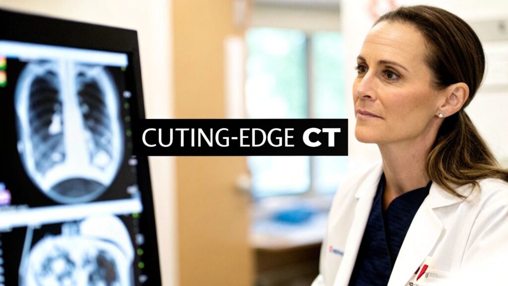
A volumetric CT scan is how the gantry acquires a volume: the table moves while the tube spins (helical / spiral), a multi-detector row grabs many slices per rotation, and reconstruction writes a stack you can reformat. This page is that scan mode. It is not volume rendering (how you paint the volume afterward).
If you meant volume rendering the visualization (MIP / DVR / transfer functions) → volume rendering of CT. If you meant 4D / gated (time as a fourth axis) → 4D CT scan. If you meant how images are acquired across modalities → acquisition of images. If you meant cone-beam → what a CBCT is.
From one slice to a volume
Godfrey Hounsfield’s 1971 scanner (EMI Mark I) could do a head. One picture took on the order of four and a half minutes. That is CT, not volumetric CT. A volume needs a continuous slab, not a handful of paused slices.
Spiral / helical CT (early 1990s) is the break: the gantry rotates without stopping while the table feeds the patient through. One breath-hold can cover a chest or an abdomen. You stop asking the patient to hold still for slice 12, then 13, then 14. Motion drops. The output is a volume you can recut in any plane.
Helical and spiral are the same geometry. Radiology says both. “Volume CT” in that vocabulary is this acquisition, not a render.
MDCT: detector rows
Multi-detector CT (MDCT) put more than one detector row on the gantry. One rotation writes many slices. Rows went 4 → 16 → 32 → 64 and up. Coverage per turn grew; scan time shrank; isotropic voxels became a protocol, not a stunt. Coronary arteries and a whole-aorta run are why those rows exist.
| Generation | Detector rows | Rotation | What you get |
|---|---|---|---|
| First practical CT (1971) | 1 | Minutes | One slice. Not a volume. |
| Helical / spiral (1990s) | 1 row, moving table | Seconds | A volume in one breath-hold |
| Early MDCT (~2000s) | 4–16 | Sub-second | Thinner slices, less stair-step |
| Modern MDCT | 64+ | Sub-second | Isotropic / near-isotropic coverage of an organ |
The mm choice on those slices — acquired vs reconstructed, cardiac 0.5 mm vs routine abdomen 3–5 mm — is CT slice thickness. This page stops at “the scanner can grab a volume.”
What happens after the photons
Detectors measure attenuation. Software turns that into slices. Iterative reconstruction (and later deep-learning recon) is the usual modern path: less noise for a given dose, or less dose for a given noise. The FBP vs IR math is 3D reconstruction from CT — not a second copy here.
Dual-energy (two kV) and photon-counting detectors are the current hardware step: count photons and their energy instead of integrating a charge. That is still acquisition. It gives you better tissue separation and, often, a lower dose. It does not paint a cinematic render. Spectral / photon-counting is a scanner feature; MIP vs DVR is a viewer feature.
What the volume is for
- Cardiology. A helical cardiac CTA is a volume of the coronaries in one or a few beats. You need the rows and the rotation time, not a pretty shader.
- Oncology / staging. A chest–abdomen–pelvis volume in one session, reformattable, comparable on follow-up.
- Emergency. Polytrauma: bone, bleed, and organs from one pass because the table never stopped.
- Neuro. A head volume you can recut — stroke, bleed, aneurysm — without re-scanning for a coronal.
4D / gated CT is the same idea with time bins (breath or ECG). That movie is 4D CT scan. A cone-beam volume from a C-arm or dental unit is CBCT, not this MDCT helical page.
Dose and data
A volume is more photons than three scout slices. Iterative recon and protocol work (kV, mA, collimation, pitch) are how you keep ALARA. The scan also writes a large series — storage and a PACS that will not choke are part of owning MDCT, not an afterthought.
This is not a volume-rendering tutorial and it is not a 4D primer. Paint the volume → volume rendering of CT. Gate it → 4D CT.
PYCAD builds products that have to treat “we scanned a volume” as a different fact from “we rendered it.” Case studies.